UNIT II TRANSACTION FLOW TESTING UNIT II TRANSACTION

UNIT – II TRANSACTION FLOW TESTING

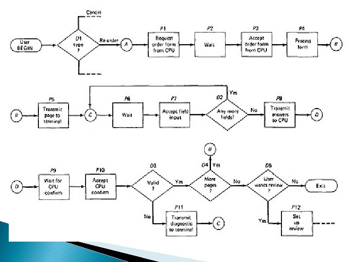
UNIT – II TRANSACTION FLOW TESTING 1. A transaction is a unit of work seen from a system user's point of view. 2. A transaction consists of a sequence of operations, some of which are performed by a system, persons or devices that are outside of the system. 3. Transaction begin with Birth-that is they are created as a result of some external act. 4. At the conclusion of the transaction's processing, the transaction is no longer in the system.

Example of a transaction: A transaction for an online information retrieval system might consist of the following steps or tasks: 1. Accept input (tentative birth) 2. Validate input (birth) 3. Transmit acknowledgement to requester 4. Do input processing 5. Search file 6. Request directions from user 7. Accept input 8. Validate input 9. Process request 10. Update file 11. Transmit output 12. Record transaction in log and clean up (death)

TRANSACTION FLOW GRAPHS: 1. Transaction flows are introduced as a representation of a system's processing. 2. The methods that were applied to control flow graphs are then used for functional testing. 3. Transaction flows and transaction flow testing are to the independent system tester what control flows are path testing are to the programmer. 4. The transaction flow graph is to create a behavioral model of the program that leads to functional testing. 5. The transaction flowgraph is a model of the structure of the system's behavior (functionality). An example of a Transaction Flow is as follows:

COMPLICATIONS: In simple cases, the transactions have a unique identity from the time they're created to the time they're completed. In many systems the transactions can give birth to others, and transactions can also merge. Births: There are three different possible interpretations of the decision symbol, or nodes with two or more out links. It can be a Decision, Biosis or a Mitosis. Decision: Here the transaction will take one alternative or the other alternative but not both. (See Figure) Biosis: Here the incoming transaction gives birth to a new transaction, and both transaction continue on their separate paths, and the parent retains it identity. (See Figure ) Mitosis: Here the parent transaction is destroyed and two new transactions are created. (See Figure)

Nodes with multiple outlinks

Mergers: Transaction flow junction points are potentially as troublesome as transaction flow splits. There are three types of junctions: (1) Ordinary Junction (2) Absorption (3) Conjugation Ordinary Junction: An ordinary junction which is similar to the junction in a control flow graph. A transaction can arrive either on one link or the other. (See Figure 3. 3 (a)) Absorption: In absorption case, the predator transaction absorbs prey transaction. The prey gone but the predator retains its identity. (See Figure 3. 3 (b)) Conjugation: In conjugation case, the two parent transactions merge to form a new daughter. In keeping with the biological flavor this case is called as conjugation. (See Figure 3. 3 (c))

Transaction Flow Junctions and Mergers

INSPECTIONS, REVIEWS AND WALKTHROUGHS: In conducting the walkthroughs, you should: 1. Discuss enough transaction types to account for 98%-99% of the transaction the system is expected to process. 2. Discuss paths through flows in functional rather than technical terms. 3. Ask the designers to relate every flow to the specification and to show that transaction, directly or indirectly, follows from the requirements.

PATH SELECTION: 1. Select a set of covering paths using the analogous (=similar or equivalent) criteria you used for structural path testing. 2. Select a covering set of paths based on functionally sensible transactions as you would for control flow graphs. 3. Try to find the most longest, strangest path from the entry to the exit of the transaction flow.

PATH SENSITIZATION: o Most of the normal paths are very easy to sensitize 80% - 95% transaction flow coverage is usually easy to achieve. o The remaining small percentage is often very difficult. PATH INSTRUMENTATION: The information of the path taken for a given transaction must be kept with that transaction and can be recorded by a central transaction dispatcher or by the individual processing modules.

BASICS OF DATA FLOW TESTING: � DATA FLOW TESTING: o Data flow testing is the name given to a family of test strategies based on selecting paths through the program's control flow in order to explore sequences of events related to the status of data objects. o For example, pick enough paths to assure that every data object has been initialized prior to use or that all defined objects have been used for something.

DATA FLOW MACHINES: o There are two types of data flow machines with different architectures. (1) Von Neumann machines (2) Multi-instruction, multi-data machines (MIMD). o Von Neumann Machine Architecture: 1. Most computers today are von-Neumann machines. 2. This architecture features interchangeable storage of instructions and data in the same memory units.

3. The Von Neumann machine Architecture executes one instruction at a time in the following, micro instruction sequence: 1. Fetch instruction from memory 2. Interpret instruction 3. Fetch operands 4. Process or Execute 5. Store result 6. Increment program counter 7. GOTO 1

o Multi-instruction, Multi-data machines (MIMD) Architecture: 1. These machines can fetch several instructions and objects in parallel. 2. They can also do arithmetic and logical operations simultaneously on different data objects. 3. The decision of how to sequence them depends on the compiler.

DATA FLOW GRAPHS: o The data flow graph is a graph consisting of nodes and directed links.

o We will use a control graph to show what happens to data objects of interest at that moment. o Our objective is to expose deviations between the data flows we have and the data flows we Data Object State and Usage: 1. Data Objects can be created, killed and used. They can be used in two distinct ways: (1) In a Calculation (2) As a part of a Control Flow Predicate.

� The following symbols denote these possibilities: 1. Defined: d - defined, created, initialized etc 2. Killed or undefined: k - killed, undefined, released etc 3. Usage: u - used for something (c - used in Calculations, p - used in a predicate)

1. Defined (d): � An object is defined explicitly when it appears in a data declaration. � Or implicitly when it appears on the left hand side of the assignment. � It is also to be used to mean that a file has been opened. � A dynamically allocated object has been allocated. � Something is pushed on to the stack. � A record written.

2. Killed or Undefined (k): � An object is killed or undefined when it is released or otherwise made unavailable. � When its contents are no longer known with certitude (with aboslute certainity / perfectness). � Release of dynamically allocated objects back to the availability pool. � Return of records. � The old top of the stack after it is popped. � An assignment statement can kill and redefine immediately. For example, if A had been previously defined and we do a new assignment such as A : = 17, we have killed A's previous value and redefined A

3. Usage (u): � A variable is used for computation (c) when it appears on the right hand side of an assignment statement. � A file record is read or written. � It is used in a Predicate (p) when it appears directly in a predicate.

DATA FLOW ANOMALIES: 1. An anomaly is denoted by a two-character sequence of actions. 2. For example, ku means that the object is killed and then used, where as dd means that the object is defined twice without an intervening usage. 3. There are nine possible two-letter combinations for d, k and u. some are bugs, some are suspicious, and some are okay.

0. dd : - probably harmless but suspicious. Why define the object twice without an intervening usage? 1. dk : - probably a bug. Why define the object without using it? 2. du : - the normal case. The object is defined and then used. 3. kd : - normal situation. An object is killed and then redefined. 4. kk : - harmless but probably buggy. Did you want to be sure it was really killed? 5. ku : - a bug. the object does not exist. 6. ud : - usually not a bug because the language permits reassignment at almost any time. 7. uk : - normal situation. 8. uu : - normal situation.

A trailing dash to mean that nothing happens after the point of interest to the exit. They possible anomalies are: 0. -k : - possibly anomalous because from the entrance to this point on the path, the variable had not been defined. We are killing a variable that does not exist. 1. -d : - okay. This is just the first definition along this path. 2. -u : - possibly anomalous. Not anomalous if the variable is global and has been previously defined. 3. k- : - not anomalous. The last thing done on this path was to kill the variable. 4. d- : - possibly anomalous. The variable was defined and not used on this path. But this could be a global definition. 5. u- : - not anomalous. The variable was used but not killed on this path.

DATA FLOW ANOMALY STATE GRAPH: Data flow anomaly model prescribes that an object can be in one of four distinct states: 0. K : - undefined, previously killed, doesnot exist 1. D : - defined but not yet used for anything 2. U : - has been used for computation or in predicate 3. A : - anomalous These capital letters (K, D, U, A) denote the state of the variable and should not be confused with the program action, denoted by lower case letters.

Unforgiving Data - Flow Anomaly Flow Graph: Unforgiving model, in which once a variable becomes anomalous it can never return to a state of grace. Figure 3. 5: Unforgiving Data Flow Anomaly State Graph

Forgiving Data - Flow Anomaly Flow Graph: Forgiving model is an alternate model where redemption (recover) from the anomalous state is possible. Figure 3. 6: Forgiving Data Flow Anomaly State Graph

DATA FLOW MODEL: The data flow model is based on the program's control flow graph 0. To every statement there is a node, whose name is unique. Every node has at least one outlink and at least one inlink except for exit nodes and entry nodes. 1. Exit nodes are dummy nodes placed at the outgoing arrowheads of exit statements (e. g. , END, RETURN), to complete the graph. Similarly, entry nodes are dummy nodes placed at entry statements (e. g. , BEGIN) for the same reason. 2. The outlink of simple statements (statements with only one outlink) are weighted by the proper sequence of data-flow actions for that statement

3. Predicate nodes (e. g. , IF-THEN-ELSE, DO WHILE, CASE) are weighted with the p - use(s) on every outlink, appropriate to that outlink. 4. Every sequence of simple statements (e. g. , a sequence of nodes with one inlink and one outlink) can be replaced by a pair of nodes that has, as weights on the link between them, the concatenation of link weights. 5. If there are several data-flow actions on a given link for a given variable, then the weight of the link is denoted by the sequence of actions on that link for that variable. 6. Conversely, a link with several data-flow actions on it can be replaced by a succession of equivalent links, each of which has at most one data-flow action for any variable.

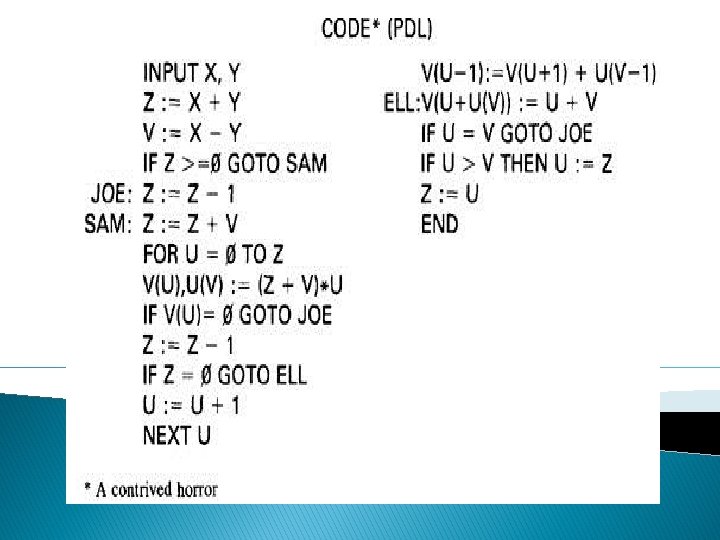
Figure 3. 8: Unannotated flowgraph for example program Figure 3. 9: Control flowgraph annotated for X and Y data flows.

Figure 3. 10: Control flowgraph annotated for Z data flow. Figure 3. 11: Control flowgraph annotated for V data flow.

STRATEGIES OF DATA FLOW TESTING: o Data Flow Testing Strategies are structural strategies. o In contrast to the path-testing strategies, data-flow strategies take into account what happens to data objects on the links in addition to the raw connectivity of the graph. o In other words, data flow strategies require data-flow link weights (d, k, u, c, p). o Data Flow Testing Strategies are based on selecting test path segments (also called sub paths) that satisfy some characteristic of data flows for all data objects. o For example, all sub paths that contain a d (or u, k, du, dk).

1. Definition-Clear Path Segment, with respect to variable X, is a connected sequence of links such that X is (possibly) defined on the first link and not redefined or killed on any subsequent link of that path segment. In Figure 3. 10, The following path segments are definition-clear: (1, 3, 4), (1, 3, 5), (5, 6, 7, 4), (7, 8, 9, 6, 7), (7, 8, 9, 10), (7, 8, 10, 11). 2. Loop-Free Path Segment is a path segment for which every node in it is visited atmost once. For Example, path (4, 5, 6, 7, 8, 10) in Figure 3. 10 is loop free, but path (10, 11, 4, 5, 6, 7, 8, 10, 11, 12) is not because nodes 10 and 11 are each visited twice.

3. Simple path segment is a path segment in which at most one node is visited twice. For example, in Figure 3. 10, (7, 4, 5, 6, 7) is a simple path segment. A simple path segment is either loop-free or if there is a loop, only one node is involved. 4. A du path from node i to k is a path segment such that if the last link has a computational use of X, then the path is simple and definition-clear; if the penultimate (last but one) node is j - that is, the path is (i, p, q, . . . , r, s, t, j, k) and link (j, k) has a predicate use then the path from i to j is both loop-free and definition-clear.

Strategies 1. All du-paths E. G Path segments (1, 3) (1, 3, 4) (1, 3, 5) 2. All-Uses strategy E. G Path segments (3, 4, 5) (3, 5) 3. All p-Uses/some c-Uses and All c-Uses/some p. Uses APU+C E. G (3, 4, 5) ACU+P E. G(3, 4, 5, 6, 7)

4. All definitions strategy 5. All predicate-uses, all computational uses strategy ORDERING THE STRATEGIES:

SLICING AND DICING: o A (static) program slice is a part of a program (e. g. , a selected set of statements) defined with respect to a given variable X (where X is a simple variable or a data vector) and a statement i: it is the set of all statements that could (potentially, under static analysis) affect the value of X at statement i - where the influence of a faulty statement could result from an improper computational use or predicate use of some other variables at prior statements

A program dice is a part of a slice in which all statements which are known to be correct have been removed. In other words, a dice is obtained from a slice by incorporating information obtained through testing or experiment (e. g. , debugging).