Particle Filtering in Network Tomography Mark Coates Mc

Particle Filtering in Network Tomography Mark Coates Mc. Gill University

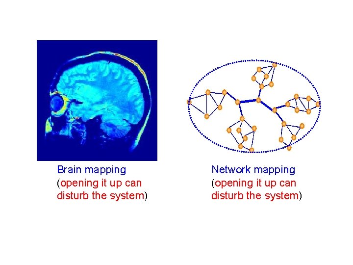
Brain mapping (opening it up can disturb the system) Network mapping (opening it up can disturb the system)

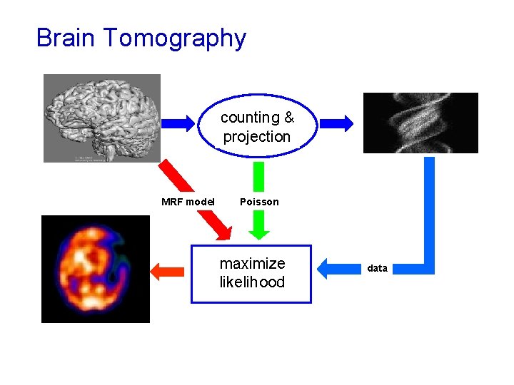
Brain Tomography unknown object statistical& counting projection model prior knowledge MRF model Maximum likelihood estimate measurements physics Poisson maximize likelihood data

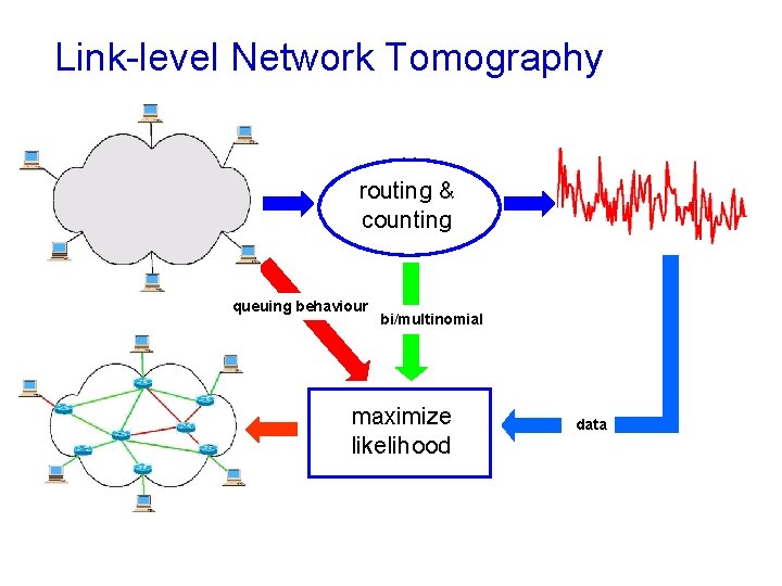
Link-level Network Tomography unknown object routing & statistical counting model queuing behaviour Maximum likelihood estimate measurements bi/multinomial physics maximize likelihood data

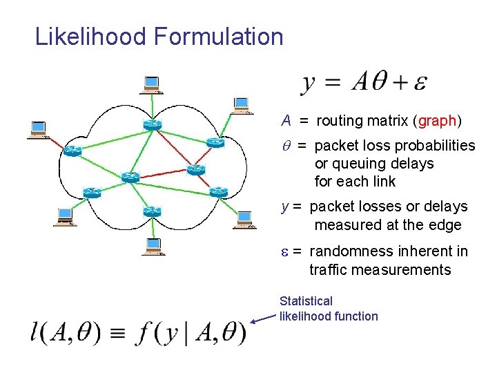
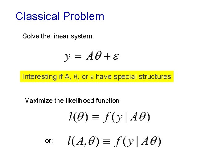
Likelihood Formulation A = routing matrix (graph) = packet loss probabilities or queuing delays for each link y = packet losses or delays measured at the edge = randomness inherent in traffic measurements Statistical likelihood function

Classical Problem Solve the linear system Interesting if A, , or have special structures Maximize the likelihood function or:

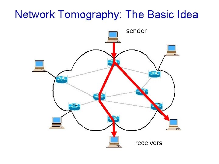
Network Tomography: The Basic Idea sender receivers

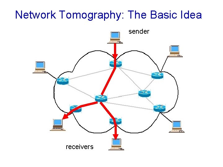
Network Tomography: The Basic Idea sender receivers

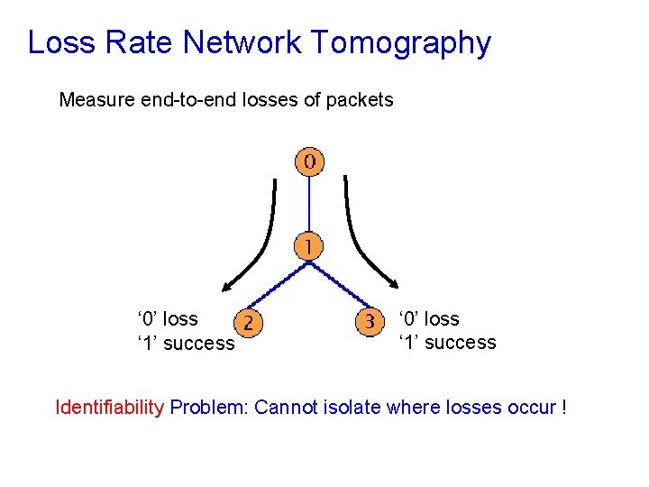
Loss Rate Network Tomography Measure end-to-end losses of packets ‘ 0’ loss ‘ 1’ success Identifiability Problem: Cannot isolate where losses occur !

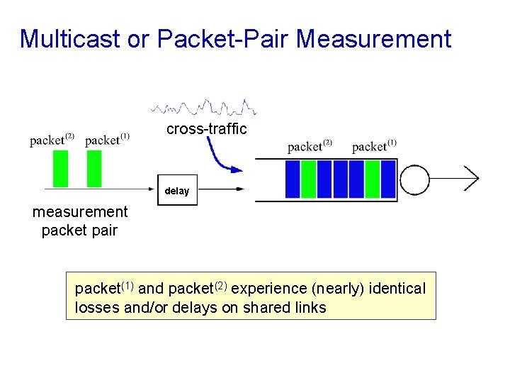
Multicast or Packet-Pair Measurement cross-traffic delay measurement packet pair packet(1) and packet(2) experience (nearly) identical losses and/or delays on shared links

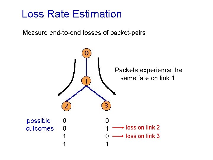
Loss Rate Estimation Measure end-to-end losses of packet-pairs Packets experience the same fate on link 1 possible outcomes 0 0 1 1 0 1 loss on link 2 loss on link 3

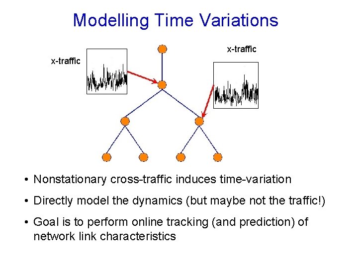
Modelling Time Variations x-traffic • Nonstationary cross-traffic induces time-variation • Directly model the dynamics (but maybe not the traffic!) • Goal is to perform online tracking (and prediction) of network link characteristics

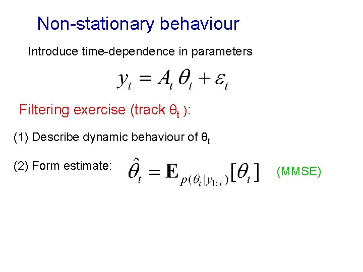
Non-stationary behaviour Introduce time-dependence in parameters Filtering exercise (track θt ): (1) Describe dynamic behaviour of θt (2) Form estimate: (MMSE)

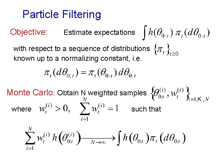
Particle Filtering Objective: Estimate expectations with respect to a sequence of distributions known up to a normalizing constant, i. e. Monte Carlo: Obtain N weighted samples where such that

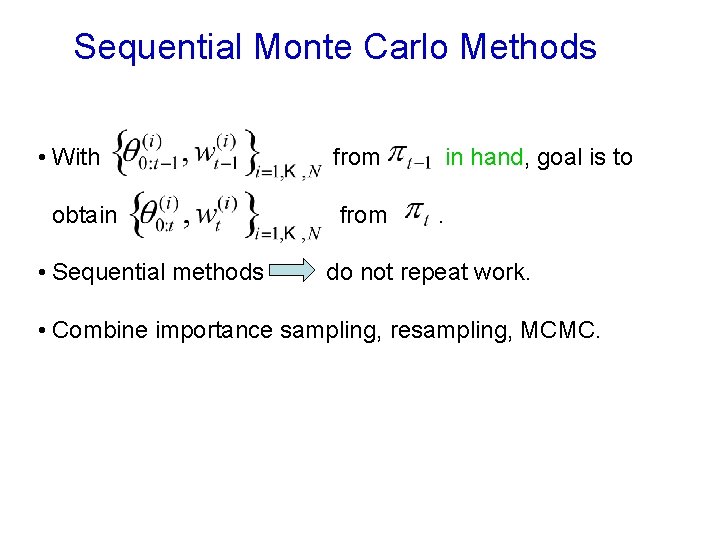
Sequential Monte Carlo Methods • With obtain • Sequential methods from in hand, goal is to. do not repeat work. • Combine importance sampling, resampling, MCMC.

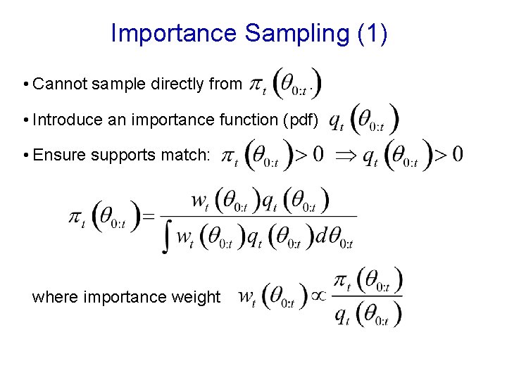
Importance Sampling (1) • Cannot sample directly from . • Introduce an importance function (pdf) • Ensure supports match: where importance weight

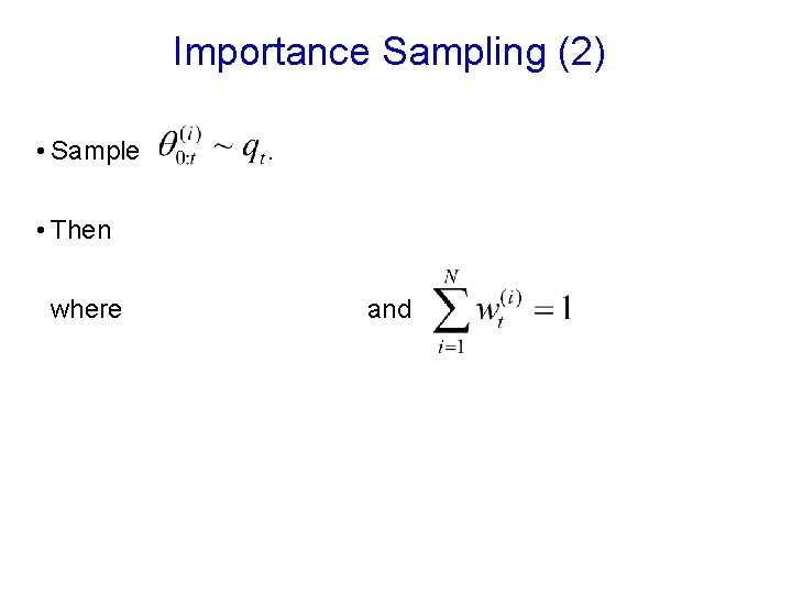
Importance Sampling (2) • Sample . • Then where and

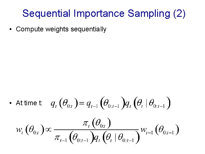
Sequential Importance Sampling (2) • Compute weights sequentially • At time t:

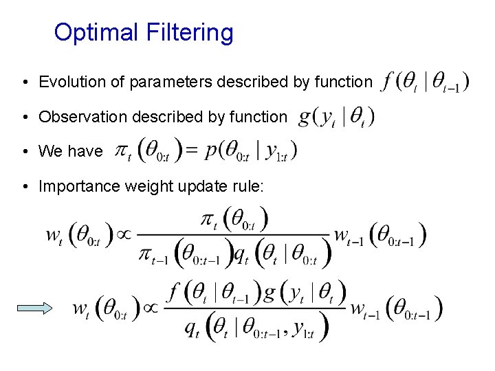
Optimal Filtering • Evolution of parameters described by function • Observation described by function • We have • Importance weight update rule:

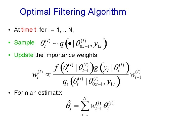
Optimal Filtering Algorithm • At time t: for i = 1, . . . , N, • Sample • Update the importance weights • Form an estimate:

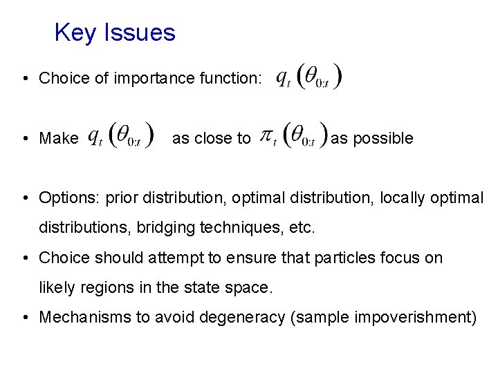
Key Issues • Choice of importance function: • Make as close to as possible • Options: prior distribution, optimal distribution, locally optimal distributions, bridging techniques, etc. • Choice should attempt to ensure that particles focus on likely regions in the state space. • Mechanisms to avoid degeneracy (sample impoverishment)

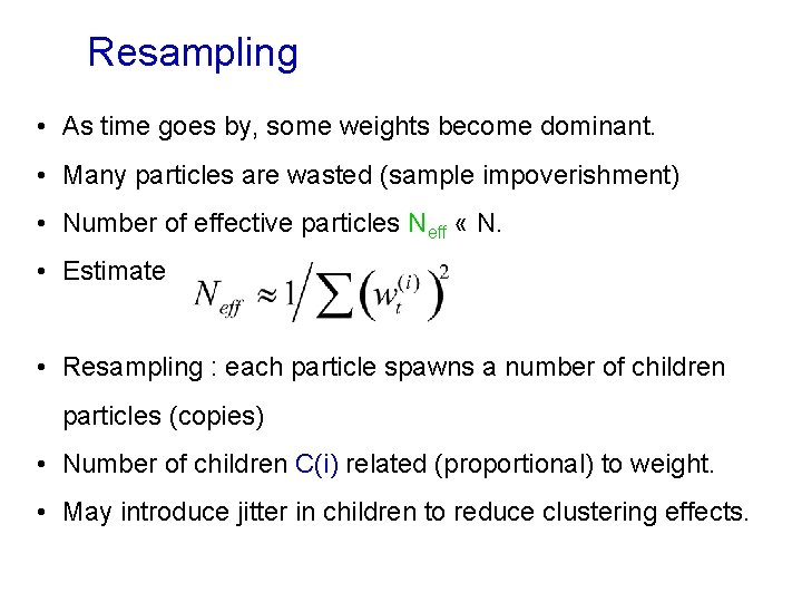
Resampling • As time goes by, some weights become dominant. • Many particles are wasted (sample impoverishment) • Number of effective particles Neff « N. • Estimate • Resampling : each particle spawns a number of children particles (copies) • Number of children C(i) related (proportional) to weight. • May introduce jitter in children to reduce clustering effects.

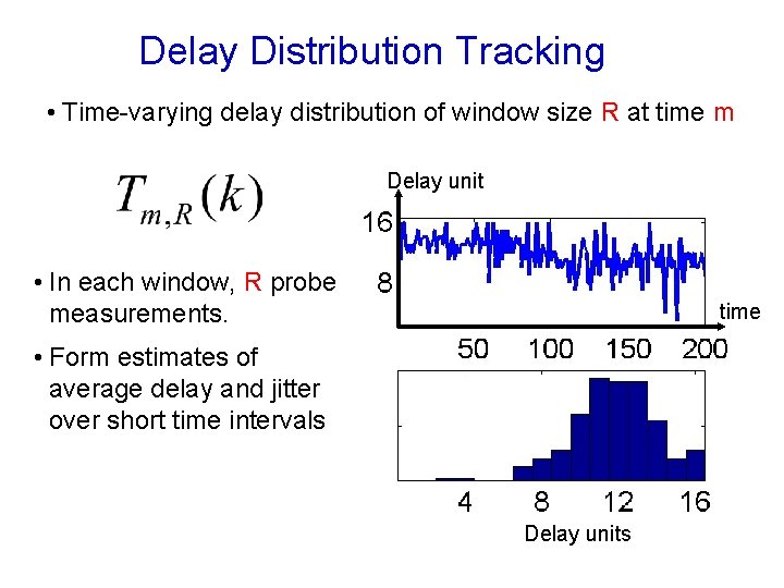
Delay Distribution Tracking • Time-varying delay distribution of window size R at time m Delay unit • In each window, R probe measurements. time • Form estimates of average delay and jitter over short time intervals Delay units

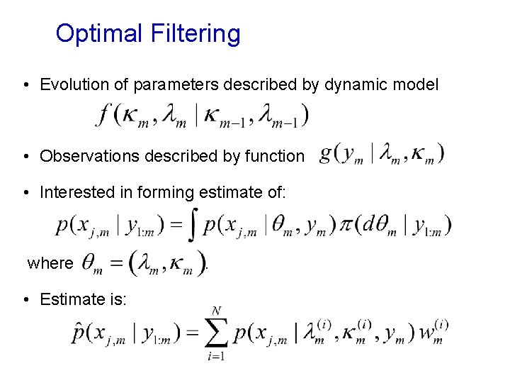
Optimal Filtering • Evolution of parameters described by dynamic model • Observations described by function • Interested in forming estimate of: where • Estimate is: .

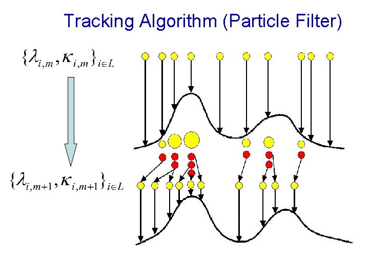
Dynamic model • Queue/traffic model: 4 4 reflected random walk on [0, max_del] Probability Delay units

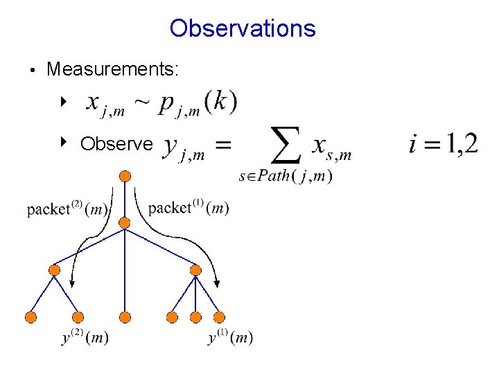
Observations • Measurements: 4 4 Observe

Tracking Algorithm (Particle Filter)

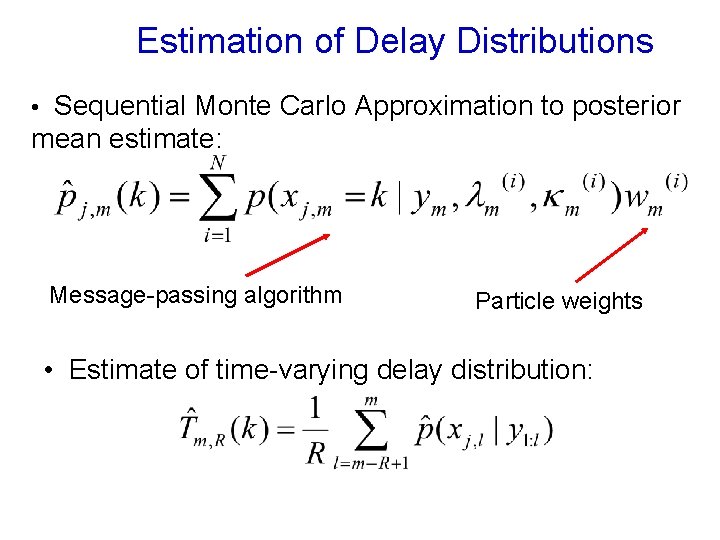
Estimation of Delay Distributions • Sequential Monte Carlo Approximation to posterior mean estimate: Message-passing algorithm Particle weights • Estimate of time-varying delay distribution:

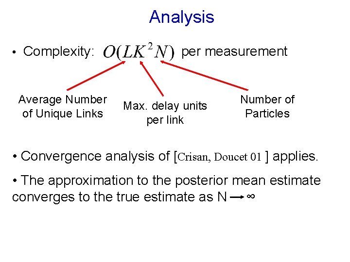
Analysis • Complexity: Average Number of Unique Links per measurement Max. delay units per link Number of Particles • Convergence analysis of [Crisan, Doucet 01 ] applies. • The approximation to the posterior mean estimate converges to the true estimate as N ∞

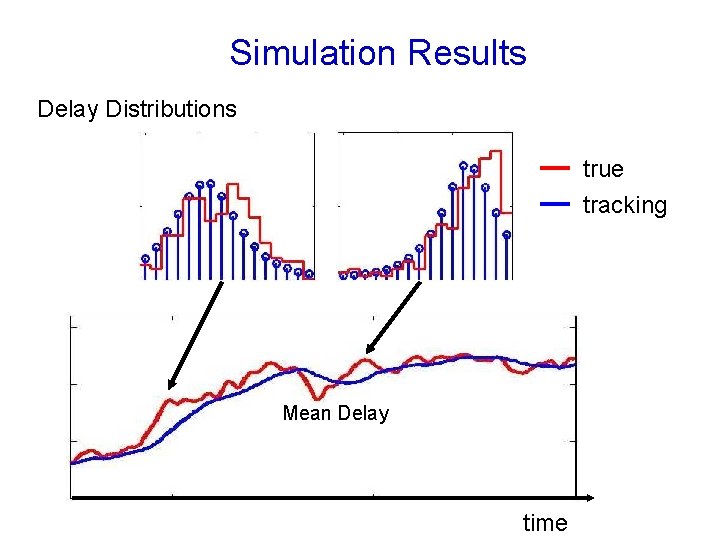
Simulation Results Delay Distributions true tracking Mean Delay time

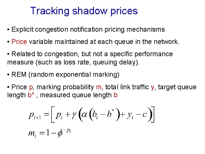
Tracking shadow prices • Explicit congestion notification pricing mechanisms • Price variable maintained at each queue in the network. • Related to congestion, but not a specific performance measure (such as loss rate, queuing delay). • REM (random exponential marking) • Price p, marking probability m, total link traffic y, target queue length b* , measured queue length b

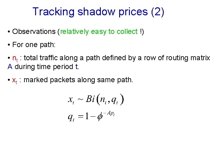
Tracking shadow prices (2) • Observations (relatively easy to collect !) • For one path: • nt : total traffic along a path defined by a row of routing matrix A during time period t. • xt : marked packets along same path.

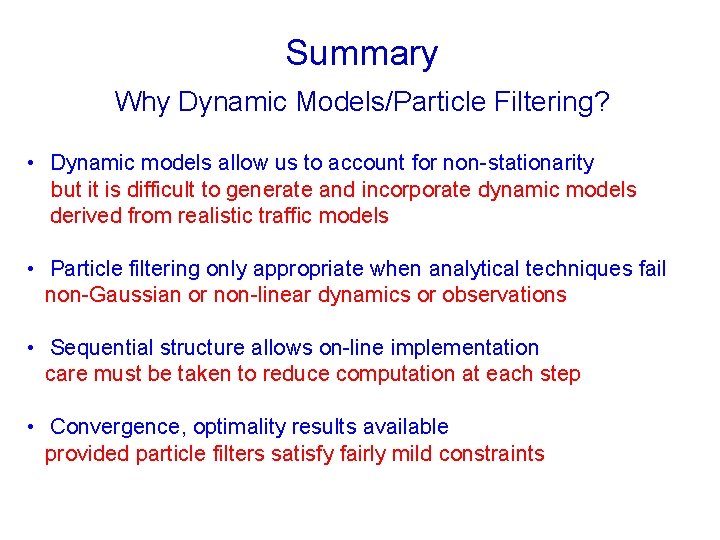
Summary Why Dynamic Models/Particle Filtering? • Dynamic models allow us to account for non-stationarity but it is difficult to generate and incorporate dynamic models derived from realistic traffic models • Particle filtering only appropriate when analytical techniques fail non-Gaussian or non-linear dynamics or observations • Sequential structure allows on-line implementation care must be taken to reduce computation at each step • Convergence, optimality results available provided particle filters satisfy fairly mild constraints