More Trees COL 106 Amit Kumar and Shweta

More Trees COL 106 Amit Kumar and Shweta Agrawal Most slides courtesy : Douglas Wilhelm Harder, MMath, UWaterloo dwharder@alumni. uwaterloo. ca

Last time. . • We saw Preorder, Inorder, Postorder traversals • Recall that in Preorder traversal, a node is visited before all its descendents • Saw recursive implementation • Saw stack implementation • Can we do better?

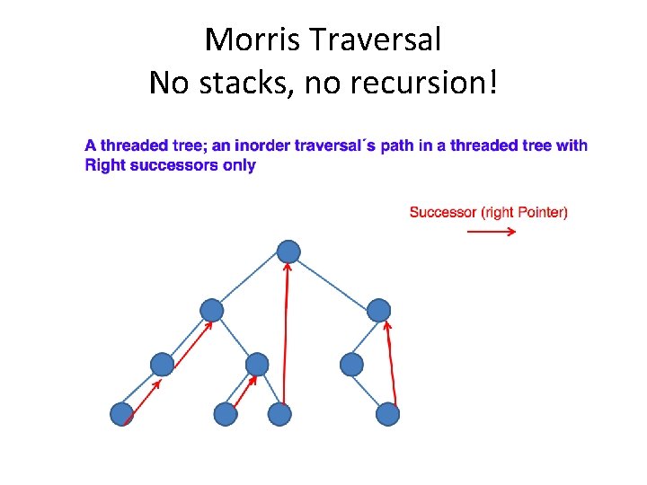
Morris Traversal No stacks, no recursion!

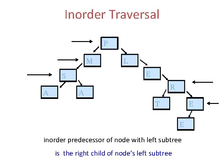
Inorder Traversal P M E S A L R A T E E inorder predecessor of node with left subtree is the right child of node’s left subtree

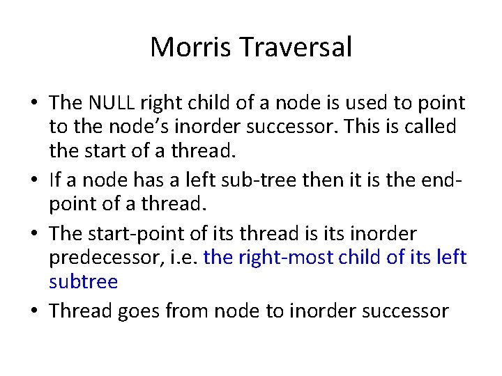
Morris Traversal • The NULL right child of a node is used to point to the node’s inorder successor. This is called the start of a thread. • If a node has a left sub-tree then it is the endpoint of a thread. • The start-point of its thread is its inorder predecessor, i. e. the right-most child of its left subtree • Thread goes from node to inorder successor

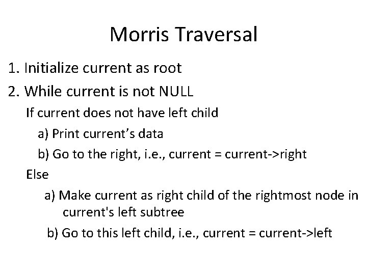
Morris Traversal 1. Initialize current as root 2. While current is not NULL If current does not have left child a) Print current’s data b) Go to the right, i. e. , current = current->right Else a) Make current as right child of the rightmost node in current's left subtree b) Go to this left child, i. e. , current = current->left

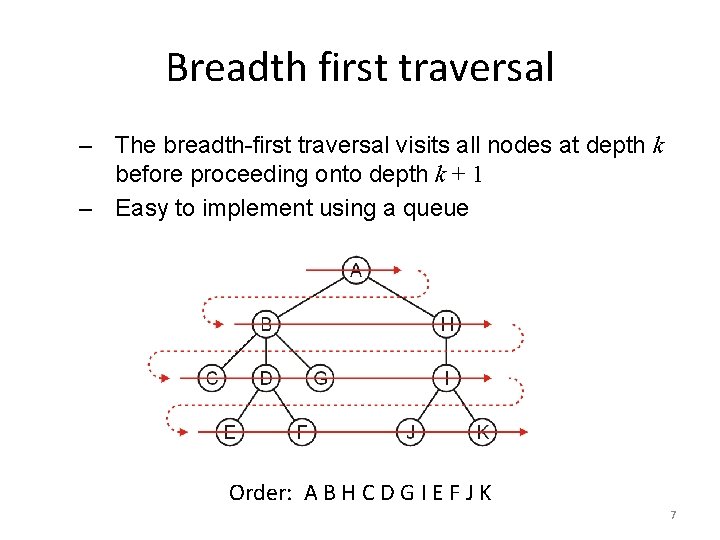
Breadth first traversal – The breadth-first traversal visits all nodes at depth k before proceeding onto depth k + 1 – Easy to implement using a queue Order: A B H C D G I E F J K 7

Breadth-First Traversal Breadth-first traversals visit all nodes at a given depth – Memory may be expensive: max nodes at given depth – Create a queue and push the root node onto queue – While the queue is not empty: • Push all of its children of the front node onto the queue • Pop the front node

Applications • Game tree for chess would need BFS • Expression printing for language processors will need pre-order / post-order DFS depending on the processor • Deleting nodes in binary search trees needs postorder traversal (will see this later)

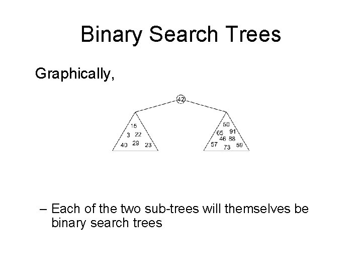
Binary Search Trees Recall that with a binary tree, we can dictate an order on the two children We will exploit this order: – Require all objects in the left sub-tree to be less than the object stored in the root node, and – Require all objects in the right sub-tree to be greater than the object in the root object

Binary Search Trees Graphically, – Each of the two sub-trees will themselves be binary search trees

Binary Search Trees Notice that we can already use this structure for searching: examine the root node and if we have not found what we are looking for: – If the object is less than what is stored in the root node, continue searching in the left sub-tree – Otherwise, continue searching the right sub-tree With a linear order, one of the following three must be true: a<b a=b a>b

Definition Thus, we define a non-empty binary search tree as a binary tree with the following properties: – The left sub-tree (if any) is a binary search tree and all elements are less than the root element, and – The right sub-tree (if any) is a binary search tree and all elements are greater than the root element

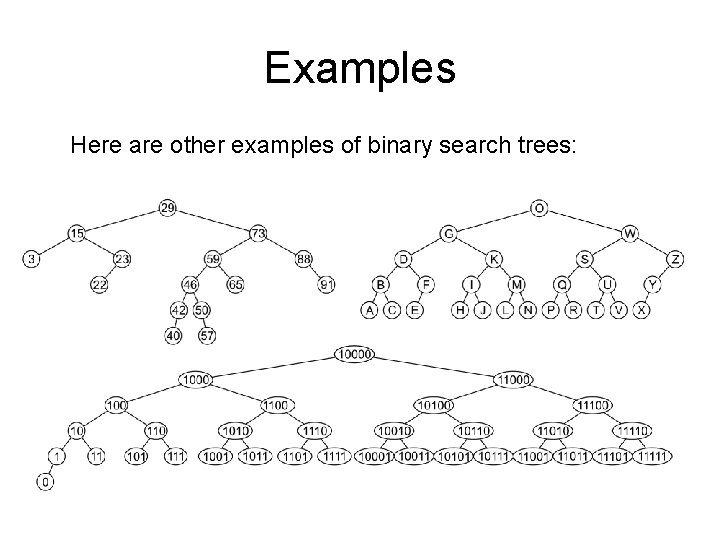
Examples Here are other examples of binary search trees:

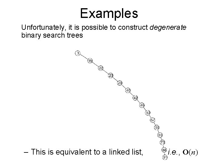
Examples Unfortunately, it is possible to construct degenerate binary search trees – This is equivalent to a linked list, i. e. , O(n)

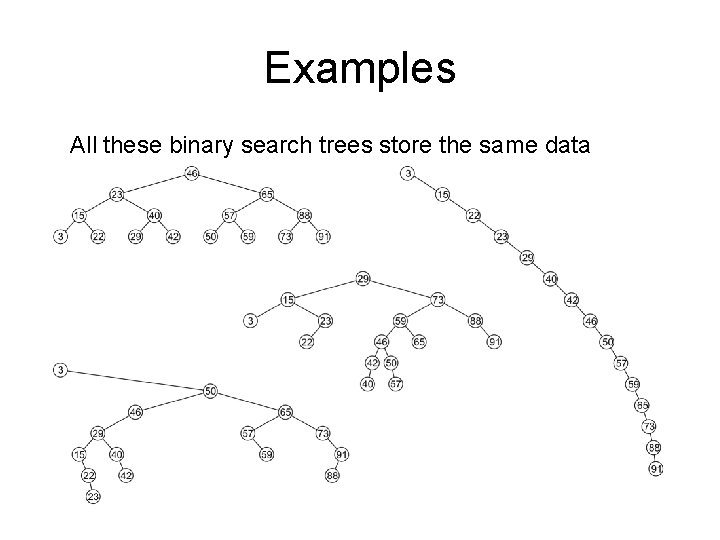
Examples All these binary search trees store the same data

Duplicate Elements We will assume that in any binary tree, we are not storing duplicate elements unless otherwise stated – In reality, it is seldom the case where duplicate elements in a container must be stored as separate entities You can always consider duplicate elements with modifications to the algorithms we will cover

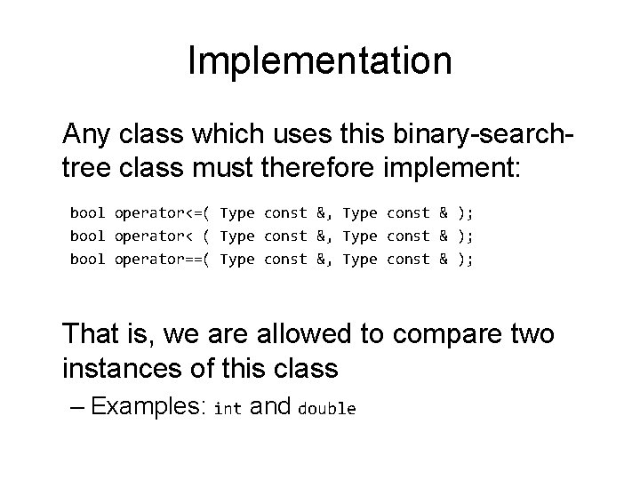
Implementation Any class which uses this binary-searchtree class must therefore implement: bool operator<=( Type const &, Type const & ); bool operator< ( Type const &, Type const & ); bool operator==( Type const &, Type const & ); That is, we are allowed to compare two instances of this class – Examples: int and double

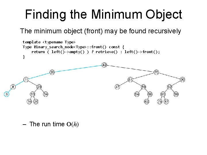
Finding the Minimum Object The minimum object (front) may be found recursively template <typename Type> Type Binary_search_node<Type>: : front() const { return ( left()->empty() ) ? retrieve() : left()->front(); } – The run time O(h)

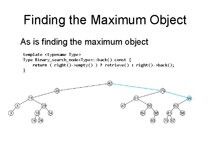
Finding the Maximum Object As is finding the maximum object template <typename Type> Type Binary_search_node<Type>: : back() const { return ( right()->empty() ) ? retrieve() : right()->back(); } – The extreme values are not necessarily leaf nodes

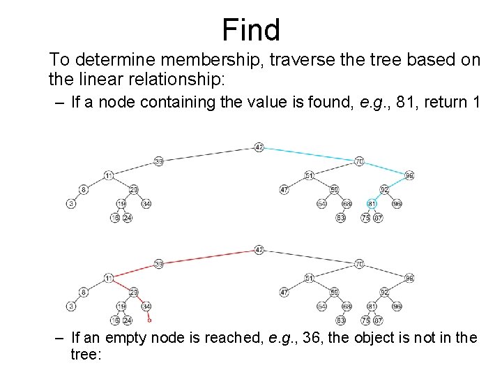
Find To determine membership, traverse the tree based on the linear relationship: – If a node containing the value is found, e. g. , 81, return 1 – If an empty node is reached, e. g. , 36, the object is not in the tree:

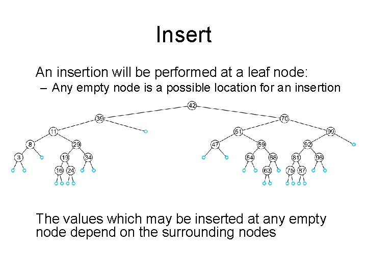
Insert Recall that a Sorted List is implicitly ordered – It does not make sense to have member functions such as push_front and push_back – Insertion will be performed by a single insert member function which places the object into the correct location

Insert An insertion will be performed at a leaf node: – Any empty node is a possible location for an insertion The values which may be inserted at any empty node depend on the surrounding nodes

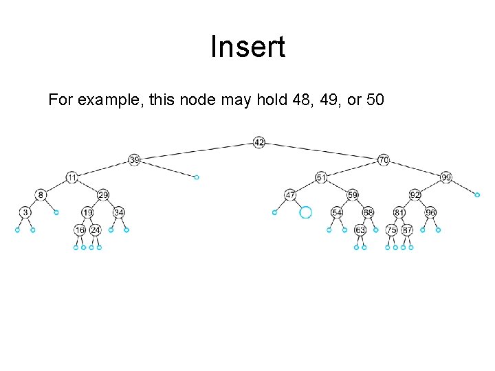
Insert For example, this node may hold 48, 49, or 50

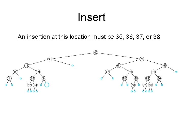
Insert An insertion at this location must be 35, 36, 37, or 38

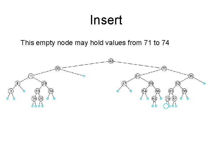
Insert This empty node may hold values from 71 to 74

Insert Like find, we will step through the tree – If we find the object already in the tree, we will return • The object is already in the binary search tree (no duplicates) – Otherwise, we will arrive at an empty node – The object will be inserted into that location – The run time is O(h)

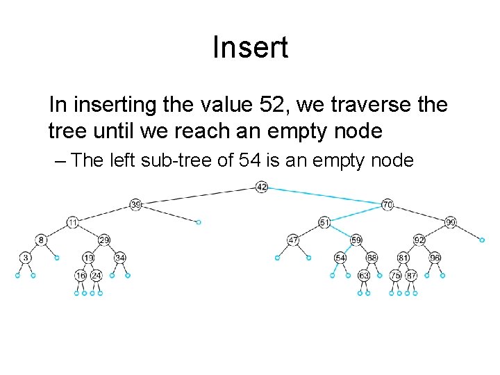
Insert In inserting the value 52, we traverse the tree until we reach an empty node – The left sub-tree of 54 is an empty node

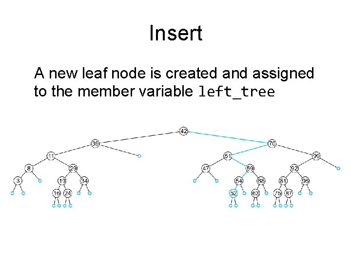
Insert A new leaf node is created and assigned to the member variable left_tree

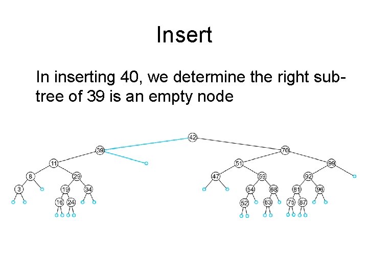
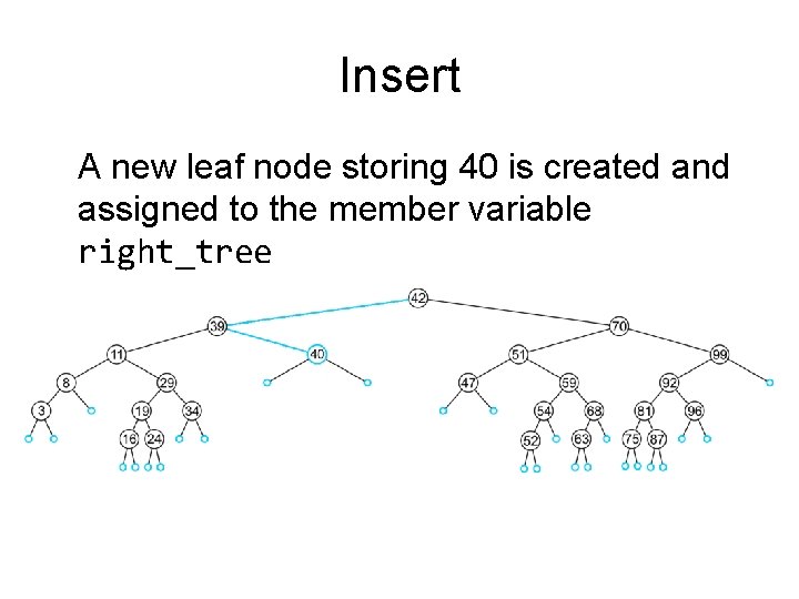
Insert In inserting 40, we determine the right subtree of 39 is an empty node

Insert A new leaf node storing 40 is created and assigned to the member variable right_tree

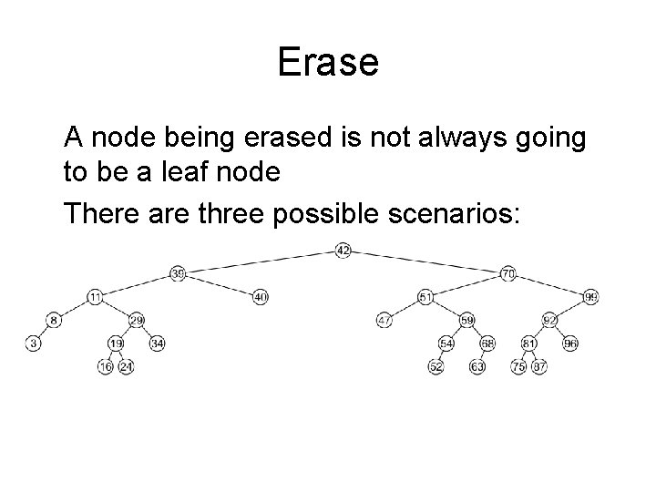
Erase A node being erased is not always going to be a leaf node There are three possible scenarios: – The node is a leaf node, – It has exactly one child, or – It has two children (it is a full node)

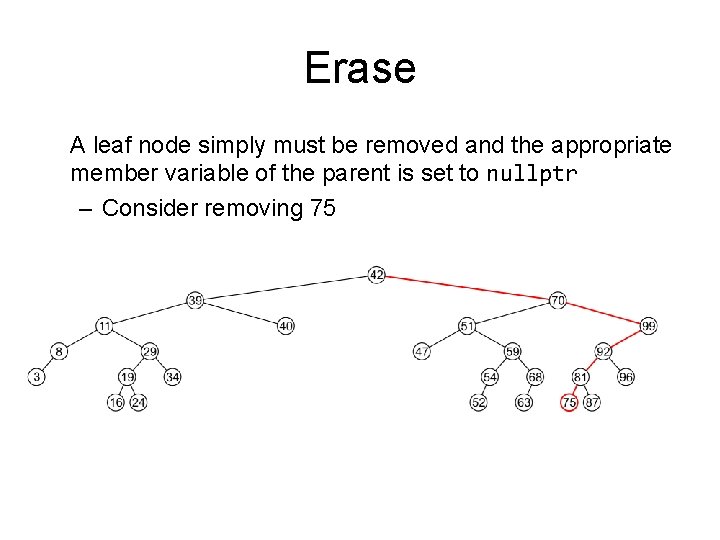
Erase A leaf node simply must be removed and the appropriate member variable of the parent is set to nullptr – Consider removing 75

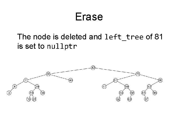
Erase The node is deleted and left_tree of 81 is set to nullptr

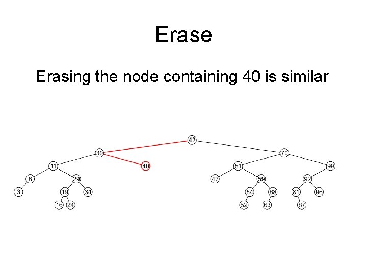
Erase Erasing the node containing 40 is similar

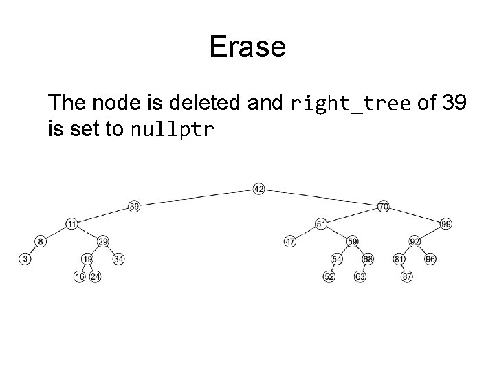
Erase The node is deleted and right_tree of 39 is set to nullptr

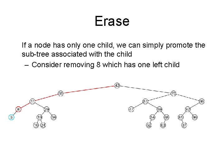
Erase If a node has only one child, we can simply promote the sub-tree associated with the child – Consider removing 8 which has one left child

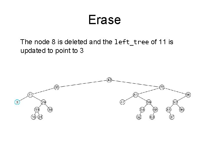
Erase The node 8 is deleted and the left_tree of 11 is updated to point to 3

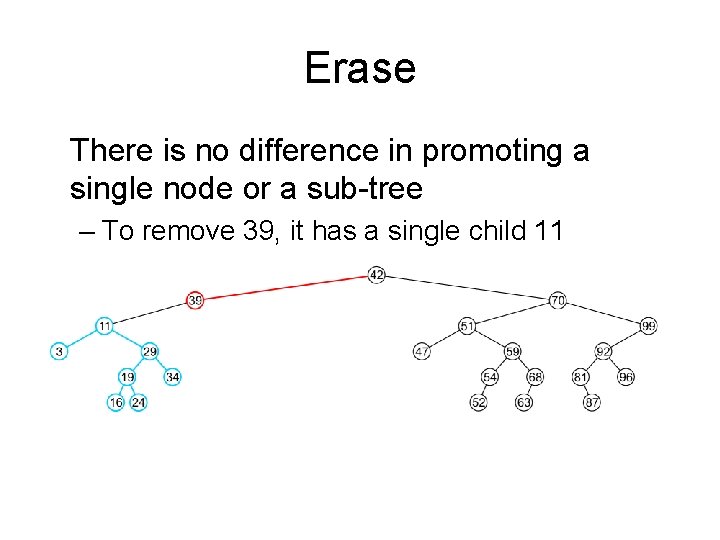
Erase There is no difference in promoting a single node or a sub-tree – To remove 39, it has a single child 11

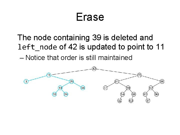
Erase The node containing 39 is deleted and left_node of 42 is updated to point to 11 – Notice that order is still maintained

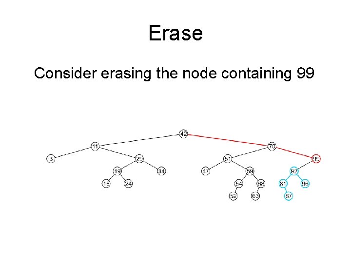
Erase Consider erasing the node containing 99

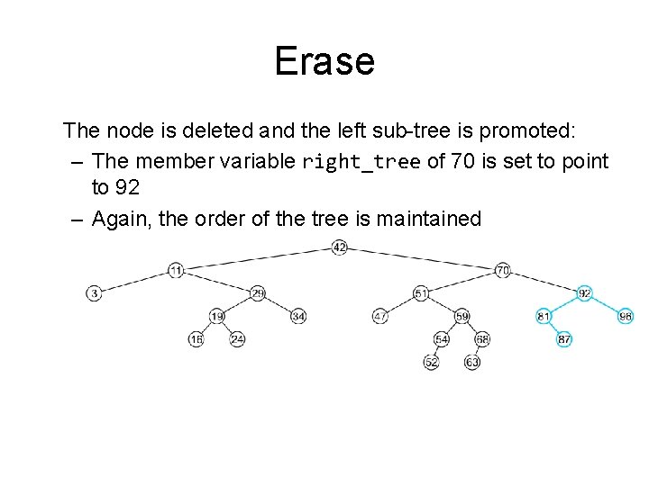
Erase The node is deleted and the left sub-tree is promoted: – The member variable right_tree of 70 is set to point to 92 – Again, the order of the tree is maintained

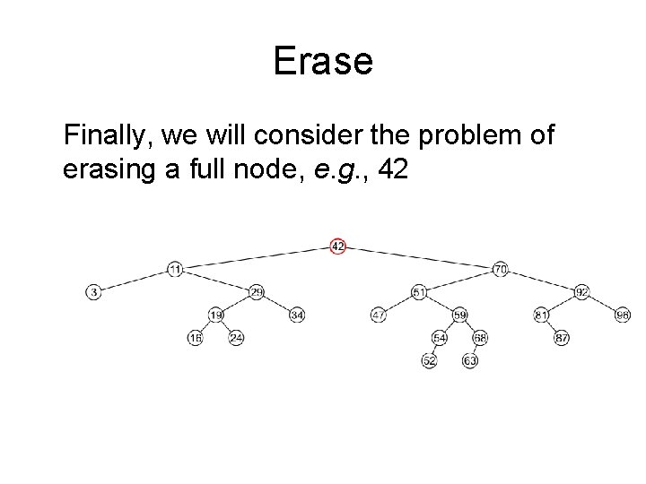
Erase Finally, we will consider the problem of erasing a full node, e. g. , 42 We will perform two operations: – Replace 42 with the minimum object in the right sub-tree – Erase that object from the right sub-tree

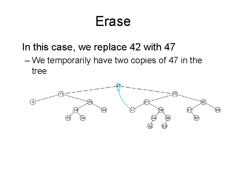
Erase In this case, we replace 42 with 47 – We temporarily have two copies of 47 in the tree

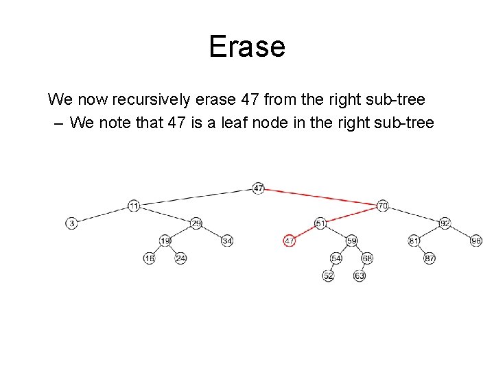
Erase We now recursively erase 47 from the right sub-tree – We note that 47 is a leaf node in the right sub-tree

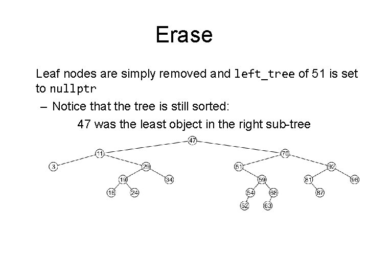
Erase Leaf nodes are simply removed and left_tree of 51 is set to nullptr – Notice that the tree is still sorted: 47 was the least object in the right sub-tree

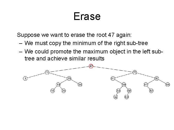
Erase Suppose we want to erase the root 47 again: – We must copy the minimum of the right sub-tree – We could promote the maximum object in the left subtree and achieve similar results

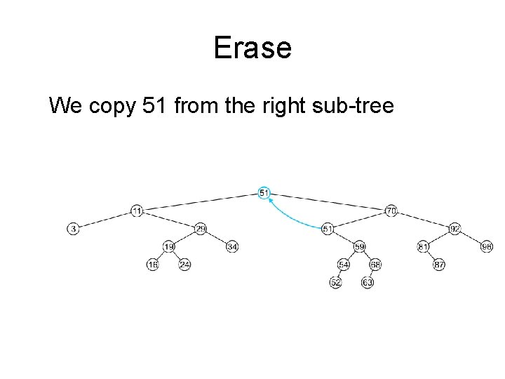
Erase We copy 51 from the right sub-tree

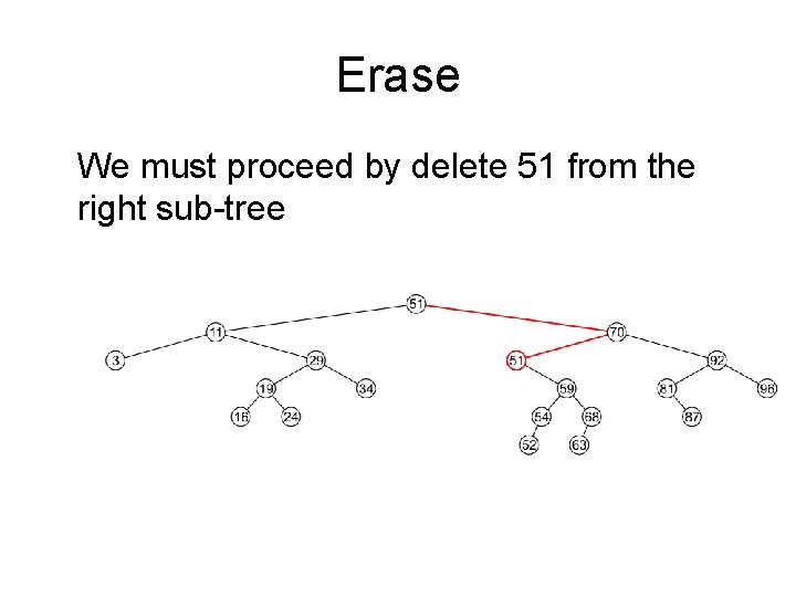
Erase We must proceed by delete 51 from the right sub-tree

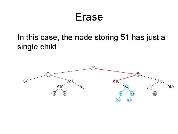
Erase In this case, the node storing 51 has just a single child

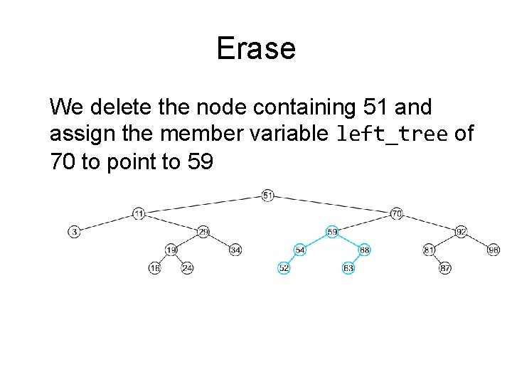
Erase We delete the node containing 51 and assign the member variable left_tree of 70 to point to 59

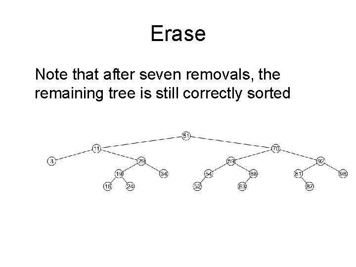
Erase Note that after seven removals, the remaining tree is still correctly sorted

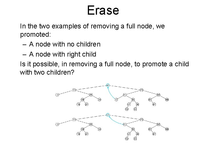
Erase In the two examples of removing a full node, we promoted: – A node with no children – A node with right child Is it possible, in removing a full node, to promote a child with two children?

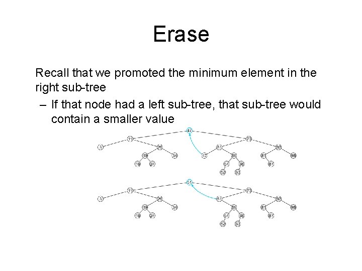
Erase Recall that we promoted the minimum element in the right sub-tree – If that node had a left sub-tree, that sub-tree would contain a smaller value

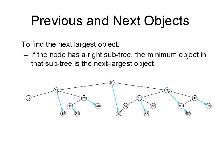
Previous and Next Objects To find the next largest object: – If the node has a right sub-tree, the minimum object in that sub-tree is the next-largest object

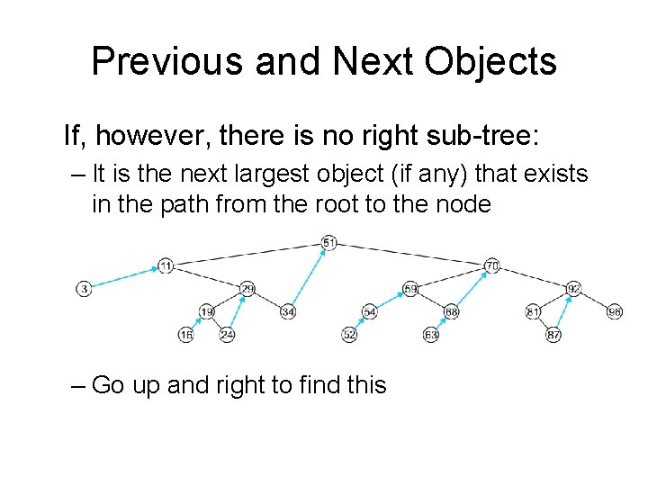
Previous and Next Objects If, however, there is no right sub-tree: – It is the next largest object (if any) that exists in the path from the root to the node – Go up and right to find this

Finding the kth Object Another operation on sorted lists may be finding the kth largest object – Recall that k goes from 0 to n – 1 – If the left-sub-tree has ℓ = k entries, return the current node, – If the left sub-tree has ℓ > k entries, return the kth entry of the left sub-tree, – Otherwise, the left sub-tree has ℓ < k entries, so return the (k – ℓ – 1)th entry of the right sub-tree