AVL Trees COL 106 Amit Kumar Shweta Agrawal

AVL Trees COL 106 Amit Kumar Shweta Agrawal Slide Courtesy : Douglas Wilhelm Harder, MMath, UWaterloo dwharder@alumni. uwaterloo. ca

Background So far … – Binary search trees store linearly ordered data – Best case height: Q(ln(n)) – Worst case height: O(n) Requirement: – Define and maintain a balance to ensure Q(ln(n)) height

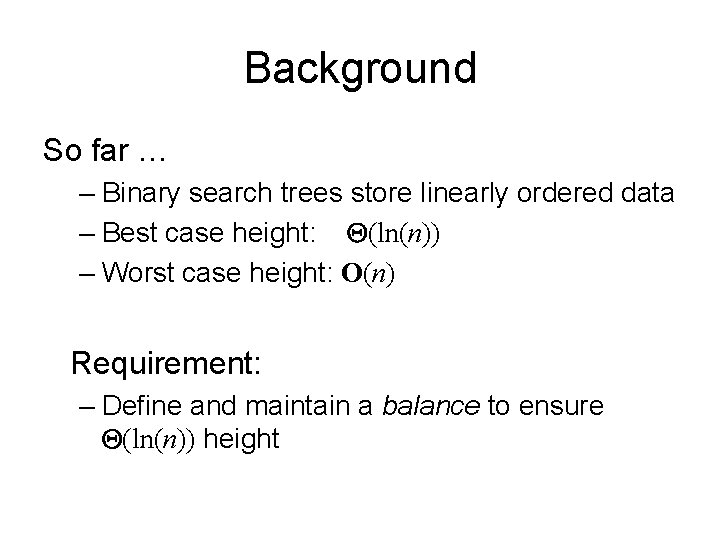
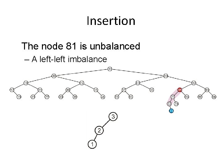
Prototypical Examples These two examples demonstrate how we can correct for imbalances: starting with this tree, add 1:

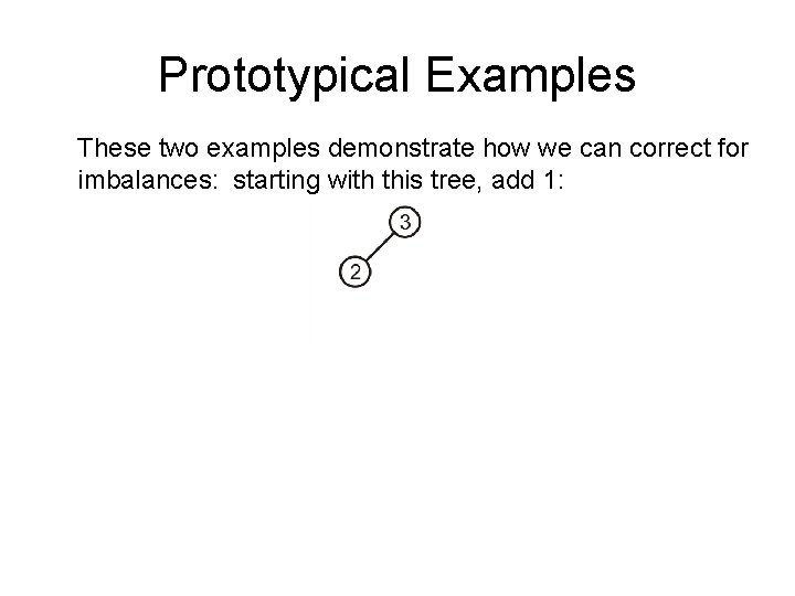
Prototypical Examples This is more like a linked list; however, we can fix this…

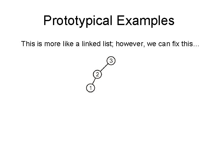
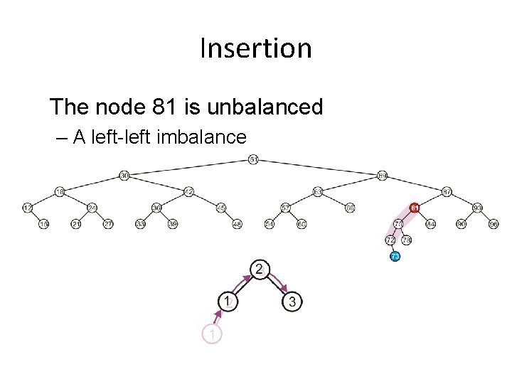
Prototypical Examples Promote 2 to the root, demote 3 to be 2’s right child, and 1 remains the left child of 2

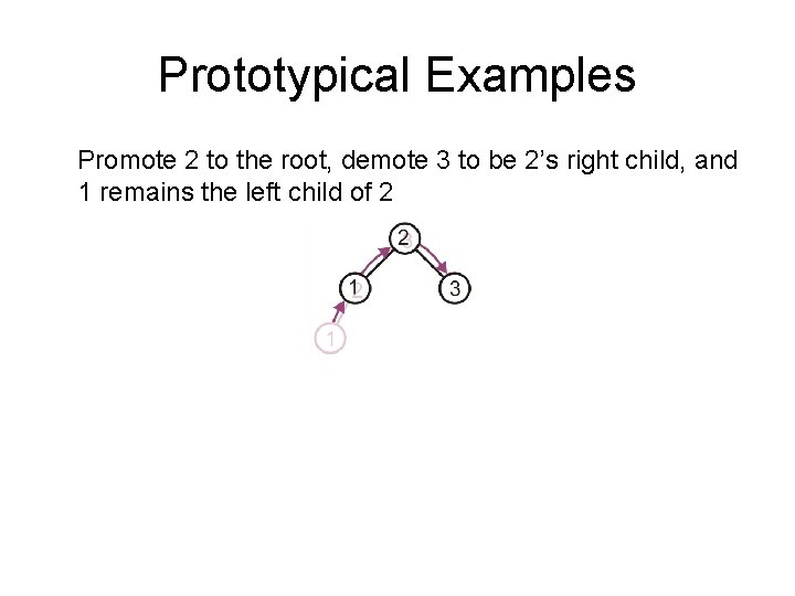
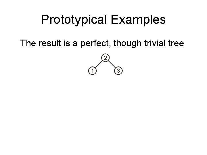
Prototypical Examples The result is a perfect, though trivial tree

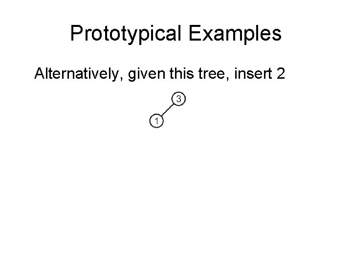
Prototypical Examples Alternatively, given this tree, insert 2

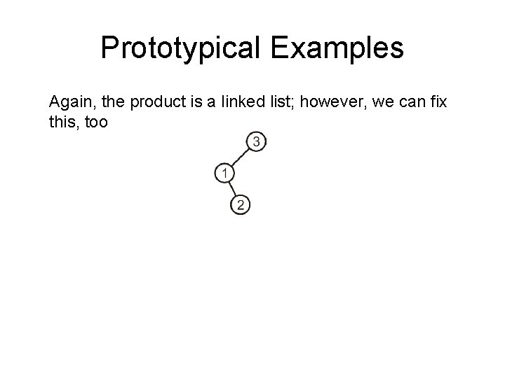
Prototypical Examples Again, the product is a linked list; however, we can fix this, too

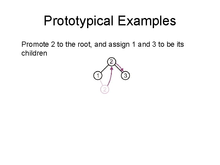
Prototypical Examples Promote 2 to the root, and assign 1 and 3 to be its children

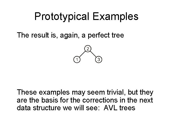
Prototypical Examples The result is, again, a perfect tree These examples may seem trivial, but they are the basis for the corrections in the next data structure we will see: AVL trees

AVL Trees We will focus on the first strategy: AVL trees – Named after Adelson-Velskii and Landis Balance is defined by comparing the height of the two sub-trees Recall: – An empty tree has height – 1 – A tree with a single node has height 0

AVL Trees A binary search tree is said to be AVL balanced if: – The difference in the heights between the left and right sub-trees is at most 1, and – Both sub-trees are themselves AVL trees

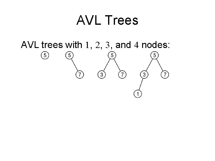
AVL Trees AVL trees with 1, 2, 3, and 4 nodes:

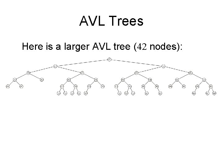
AVL Trees Here is a larger AVL tree (42 nodes):

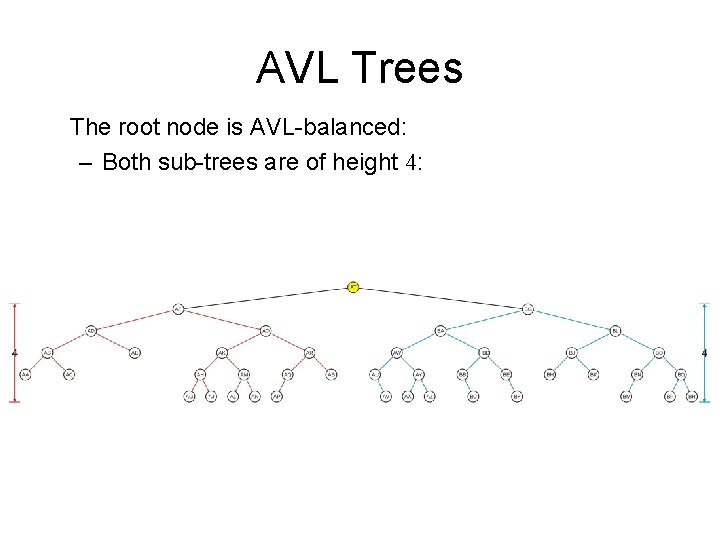
AVL Trees The root node is AVL-balanced: – Both sub-trees are of height 4:

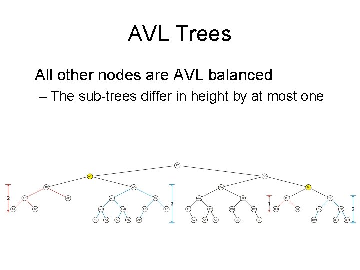
AVL Trees All other nodes are AVL balanced – The sub-trees differ in height by at most one

Height of an AVL Tree By the definition of complete trees, any complete binary search tree is an AVL tree Thus an upper bound on the number of nodes in an AVL tree of height h a perfect binary tree with 2 h + 1 – 1 nodes – What is an lower bound?

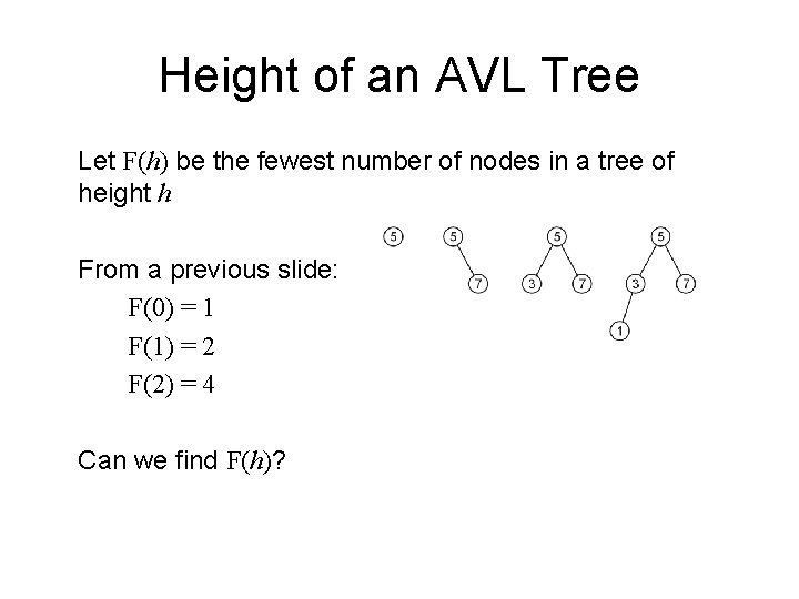
Height of an AVL Tree Let F(h) be the fewest number of nodes in a tree of height h From a previous slide: F(0) = 1 F(1) = 2 F(2) = 4 Can we find F(h)?

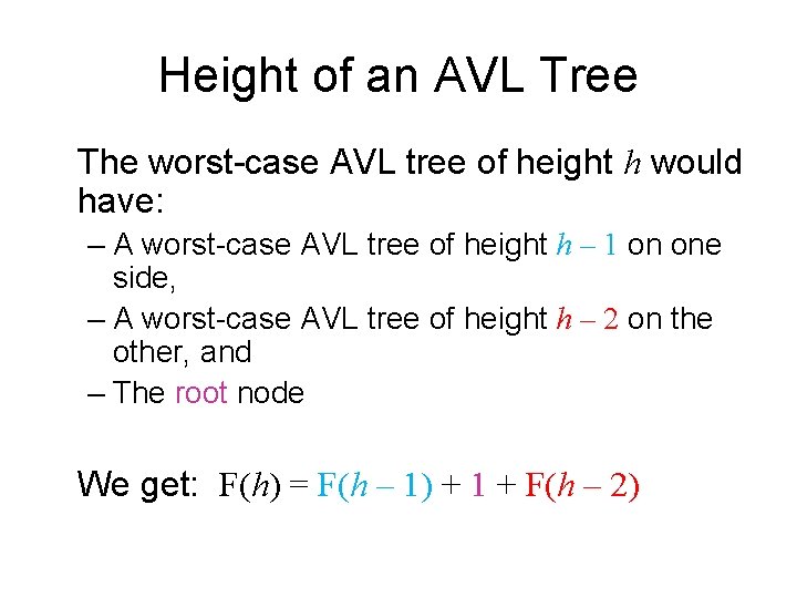
Height of an AVL Tree The worst-case AVL tree of height h would have: – A worst-case AVL tree of height h – 1 on one side, – A worst-case AVL tree of height h – 2 on the other, and – The root node We get: F(h) = F(h – 1) + 1 + F(h – 2)

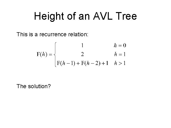
Height of an AVL Tree This is a recurrence relation: The solution?

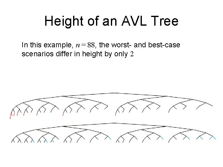
Height of an AVL Tree In this example, n = 88, the worst- and best-case scenarios differ in height by only 2

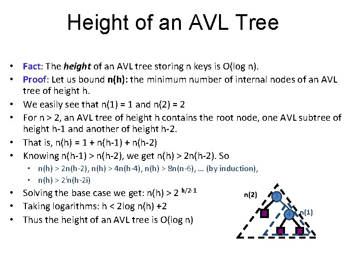
Height of an AVL Tree • Fact: The height of an AVL tree storing n keys is O(log n). • Proof: Let us bound n(h): the minimum number of internal nodes of an AVL tree of height h. • We easily see that n(1) = 1 and n(2) = 2 • For n > 2, an AVL tree of height h contains the root node, one AVL subtree of height h-1 and another of height h-2. • That is, n(h) = 1 + n(h-1) + n(h-2) • Knowing n(h-1) > n(h-2), we get n(h) > 2 n(h-2). So • n(h) > 2 n(h-2), n(h) > 4 n(h-4), n(h) > 8 n(n-6), … (by induction), • n(h) > 2 in(h-2 i) • Solving the base case we get: n(h) > 2 h/2 -1 • Taking logarithms: h < 2 log n(h) +2 • Thus the height of an AVL tree is O(log n) n(2) 3 4 n(1)

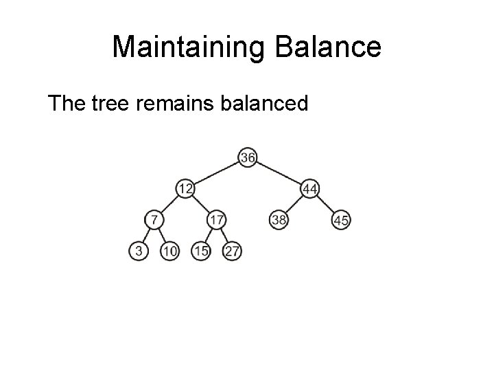
Maintaining Balance To maintain AVL balance, observe that: – Inserting a node can increase the height of a tree by at most 1 – Removing a node can decrease the height of a tree by at most 1

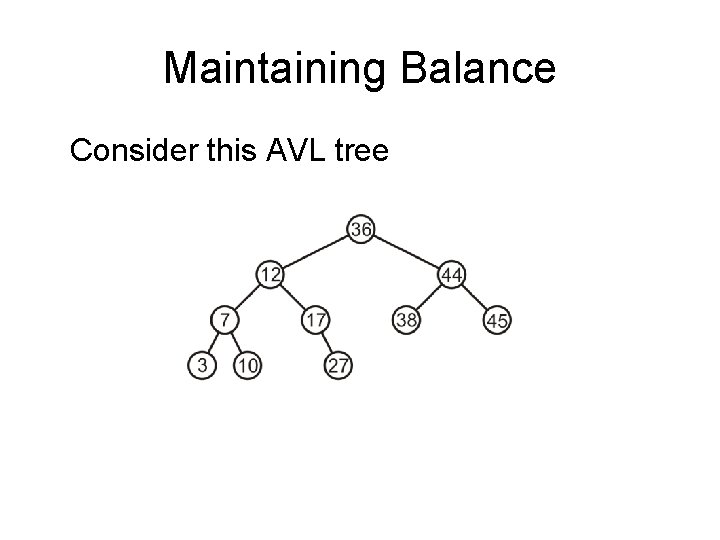
Maintaining Balance Consider this AVL tree

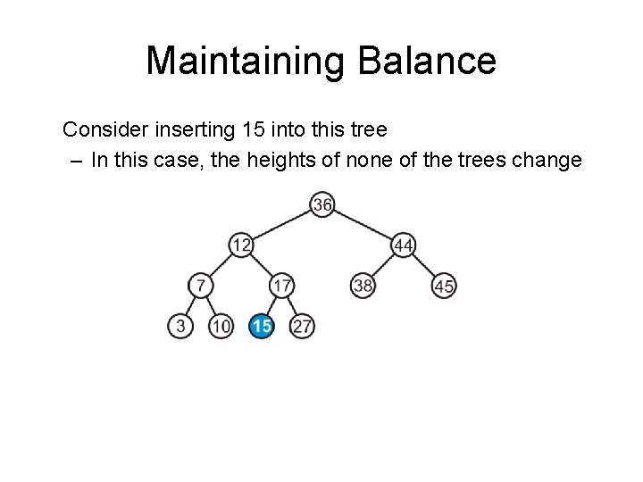
Maintaining Balance Consider inserting 15 into this tree – In this case, the heights of none of the trees change

Maintaining Balance The tree remains balanced

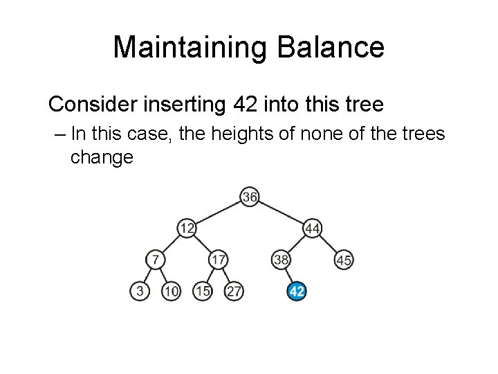
Maintaining Balance Consider inserting 42 into this tree – In this case, the heights of none of the trees change

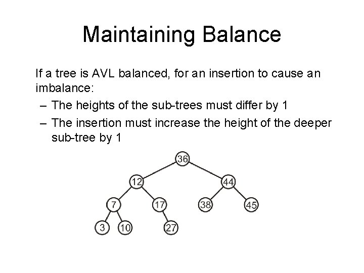
Maintaining Balance If a tree is AVL balanced, for an insertion to cause an imbalance: – The heights of the sub-trees must differ by 1 – The insertion must increase the height of the deeper sub-tree by 1

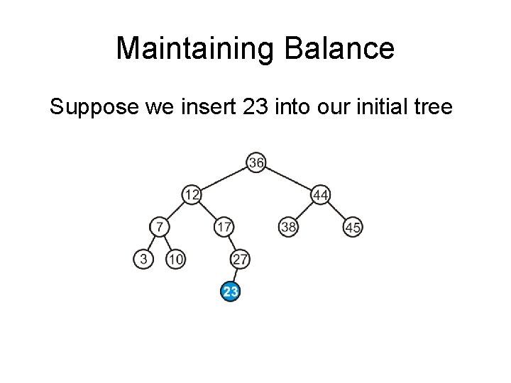
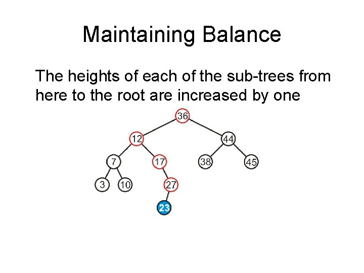
Maintaining Balance Suppose we insert 23 into our initial tree

Maintaining Balance The heights of each of the sub-trees from here to the root are increased by one

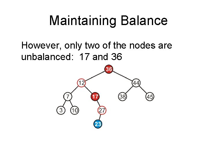
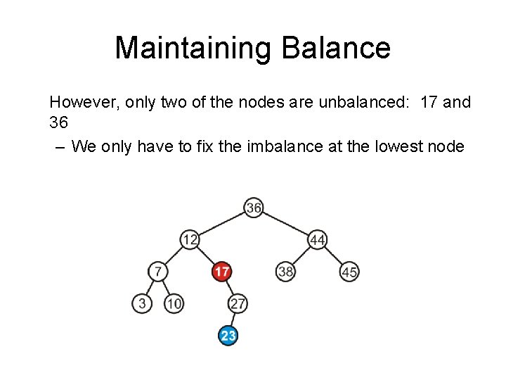
Maintaining Balance However, only two of the nodes are unbalanced: 17 and 36

Maintaining Balance However, only two of the nodes are unbalanced: 17 and 36 – We only have to fix the imbalance at the lowest node

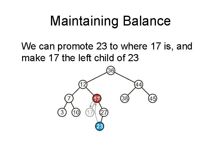
Maintaining Balance We can promote 23 to where 17 is, and make 17 the left child of 23

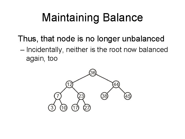
Maintaining Balance Thus, that node is no longer unbalanced – Incidentally, neither is the root now balanced again, too

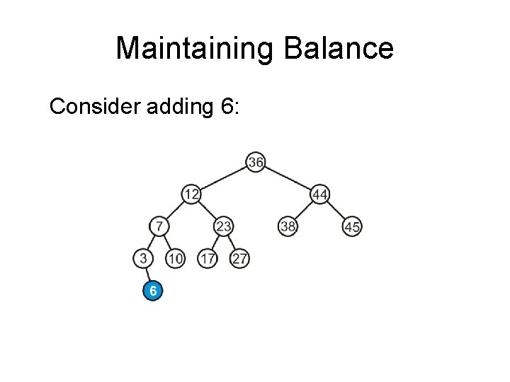
Maintaining Balance Consider adding 6:

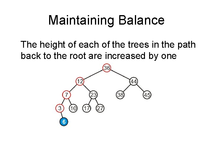
Maintaining Balance The height of each of the trees in the path back to the root are increased by one

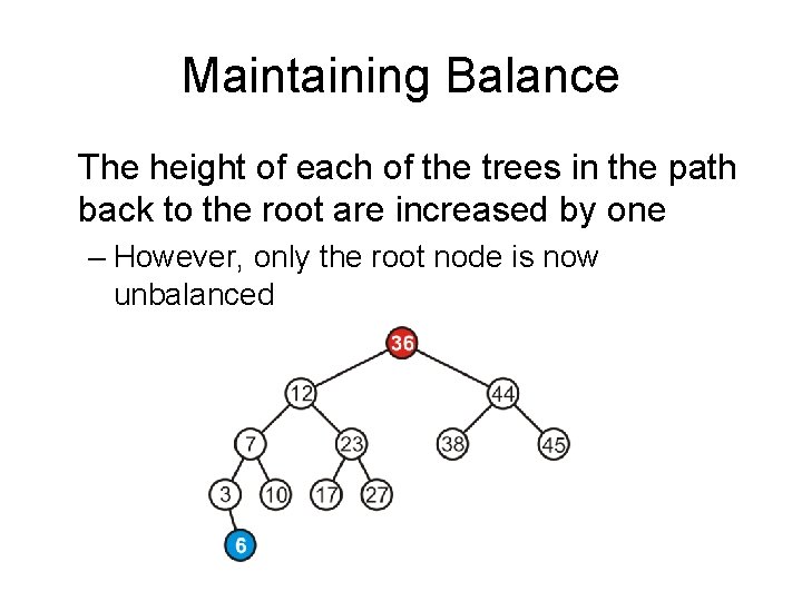
Maintaining Balance The height of each of the trees in the path back to the root are increased by one – However, only the root node is now unbalanced

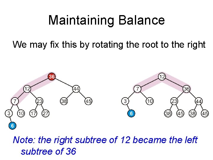
Maintaining Balance We may fix this by rotating the root to the right Note: the right subtree of 12 became the left subtree of 36

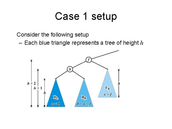
Case 1 setup Consider the following setup – Each blue triangle represents a tree of height h

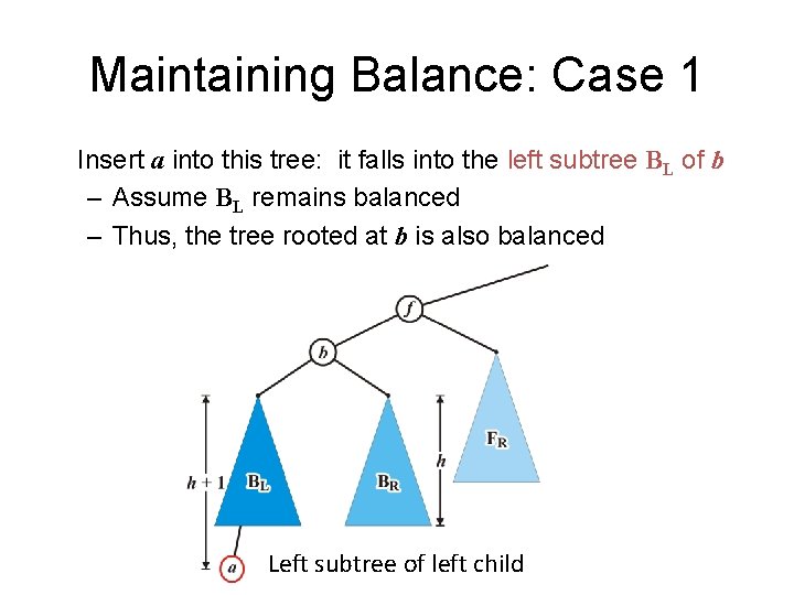
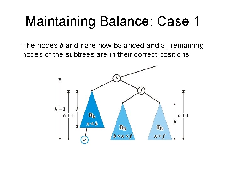
Maintaining Balance: Case 1 Insert a into this tree: it falls into the left subtree BL of b – Assume BL remains balanced – Thus, the tree rooted at b is also balanced Left subtree of left child

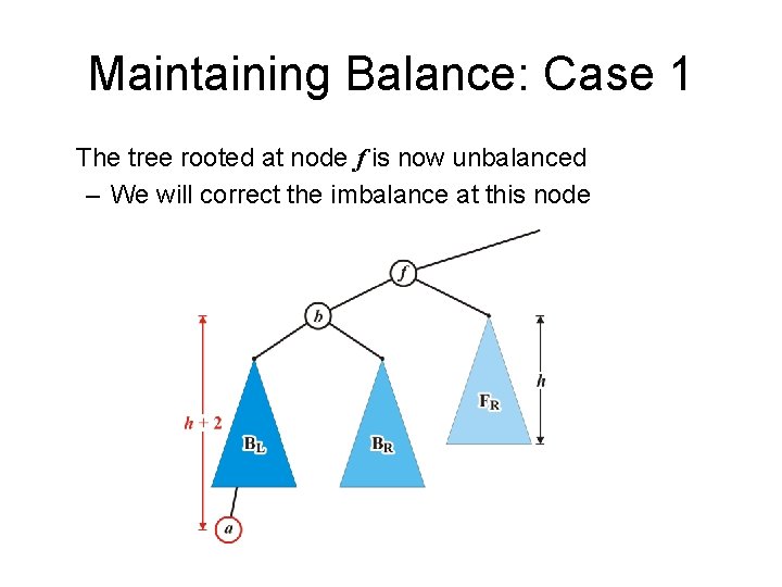
Maintaining Balance: Case 1 The tree rooted at node f is now unbalanced – We will correct the imbalance at this node

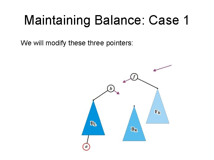
Maintaining Balance: Case 1 We will modify these three pointers:

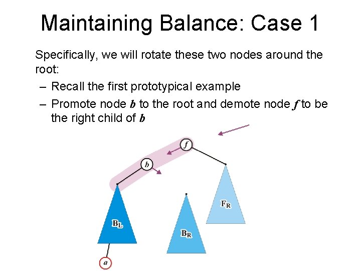
Maintaining Balance: Case 1 Specifically, we will rotate these two nodes around the root: – Recall the first prototypical example – Promote node b to the root and demote node f to be the right child of b

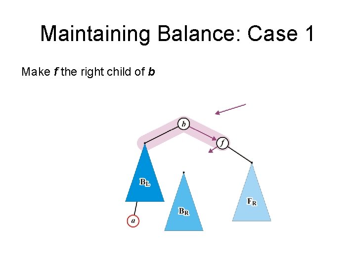
Maintaining Balance: Case 1 Make f the right child of b

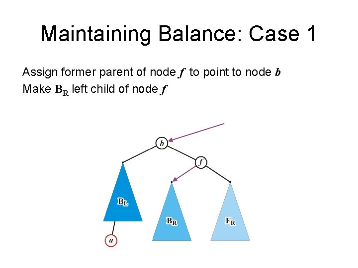
Maintaining Balance: Case 1 Assign former parent of node f to point to node b Make BR left child of node f

Maintaining Balance: Case 1 The nodes b and f are now balanced and all remaining nodes of the subtrees are in their correct positions

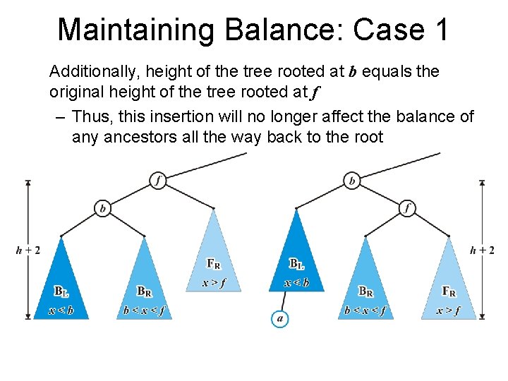
Maintaining Balance: Case 1 Additionally, height of the tree rooted at b equals the original height of the tree rooted at f – Thus, this insertion will no longer affect the balance of any ancestors all the way back to the root

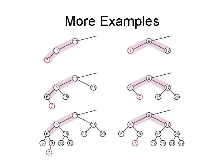
More Examples

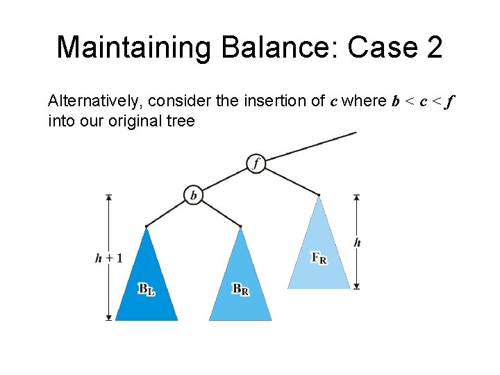
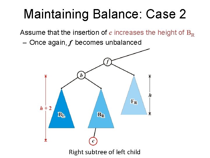
Maintaining Balance: Case 2 Alternatively, consider the insertion of c where b < c < f into our original tree

Maintaining Balance: Case 2 Assume that the insertion of c increases the height of BR – Once again, f becomes unbalanced Right subtree of left child

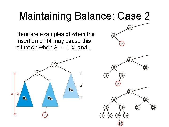
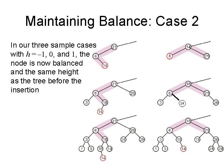
Maintaining Balance: Case 2 Here are examples of when the insertion of 14 may cause this situation when h = – 1, 0, and 1

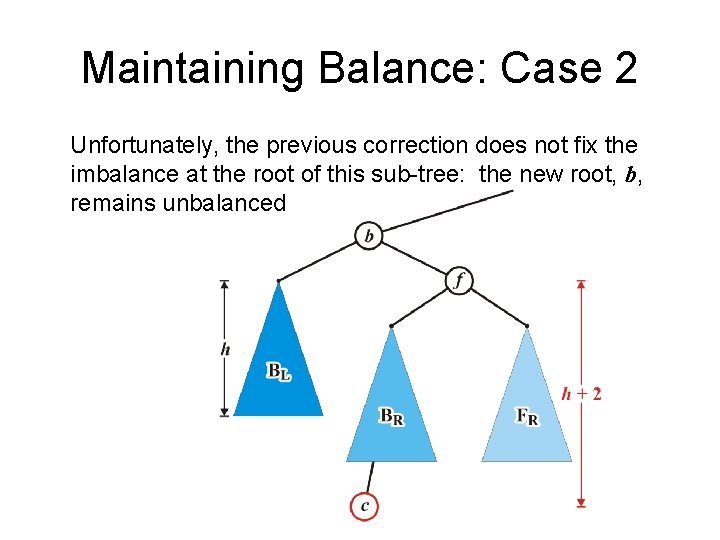
Maintaining Balance: Case 2 Unfortunately, the previous correction does not fix the imbalance at the root of this sub-tree: the new root, b, remains unbalanced

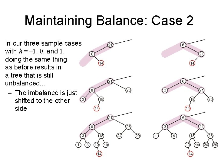
Maintaining Balance: Case 2 In our three sample cases with h = – 1, 0, and 1, doing the same thing as before results in a tree that is still unbalanced… – The imbalance is just shifted to the other side

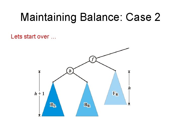
Maintaining Balance: Case 2 Lets start over …

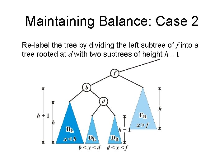
Maintaining Balance: Case 2 Re-label the tree by dividing the left subtree of f into a tree rooted at d with two subtrees of height h – 1

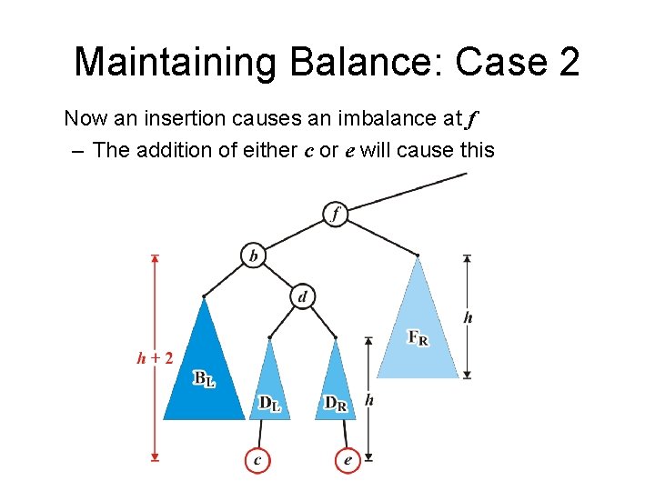
Maintaining Balance: Case 2 Now an insertion causes an imbalance at f – The addition of either c or e will cause this

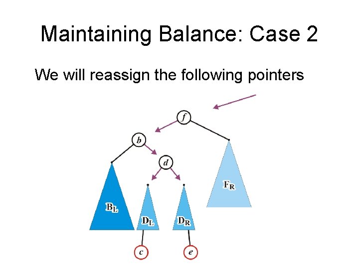
Maintaining Balance: Case 2 We will reassign the following pointers

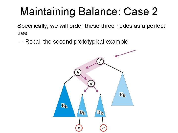
Maintaining Balance: Case 2 Specifically, we will order these three nodes as a perfect tree – Recall the second prototypical example

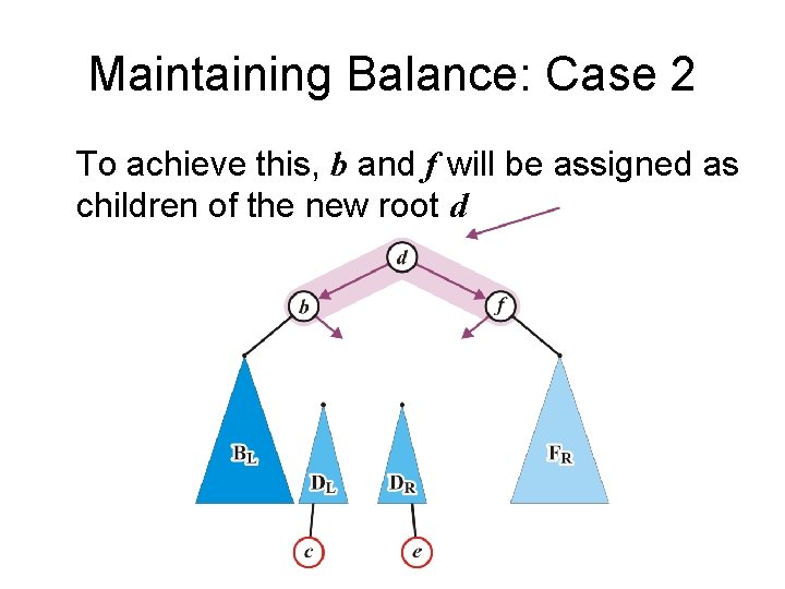
Maintaining Balance: Case 2 To achieve this, b and f will be assigned as children of the new root d

Maintaining Balance: Case 2 We also have to connect the two subtrees and original parent of f

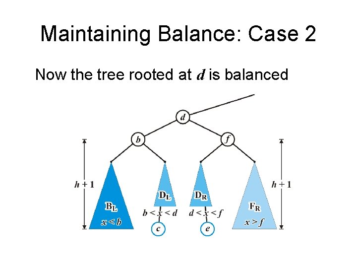
Maintaining Balance: Case 2 Now the tree rooted at d is balanced

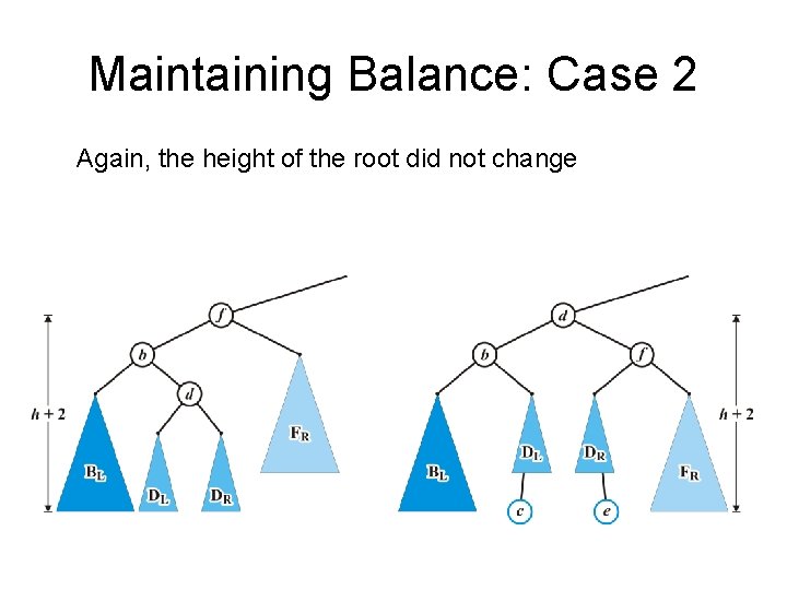
Maintaining Balance: Case 2 Again, the height of the root did not change

Maintaining Balance: Case 2 In our three sample cases with h = – 1, 0, and 1, the node is now balanced and the same height as the tree before the insertion 14

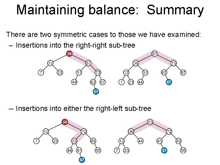
Maintaining balance: Summary There are two symmetric cases to those we have examined: – Insertions into the right-right sub-tree -- Insertions into either the right-left sub-tree

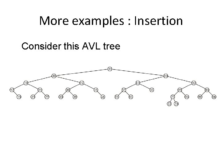
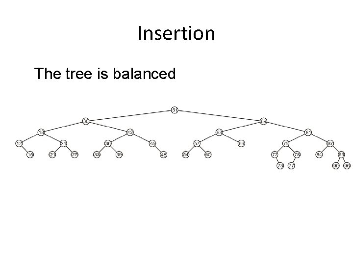
More examples : Insertion Consider this AVL tree

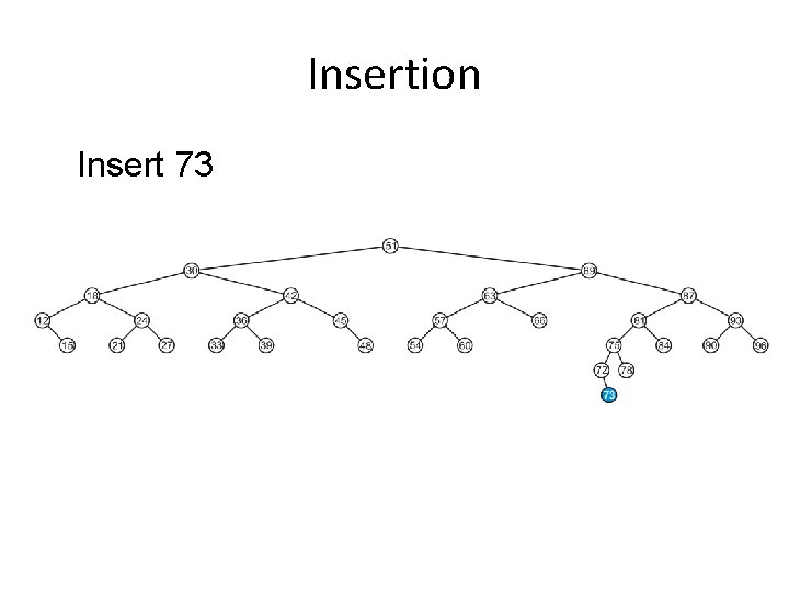
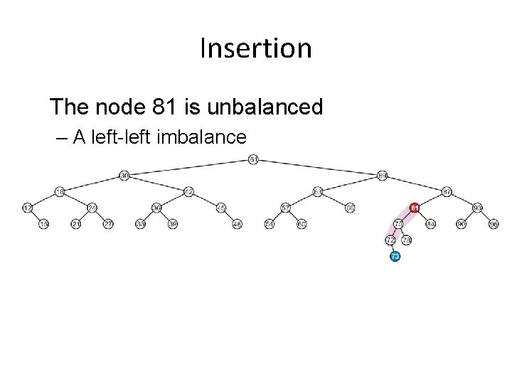
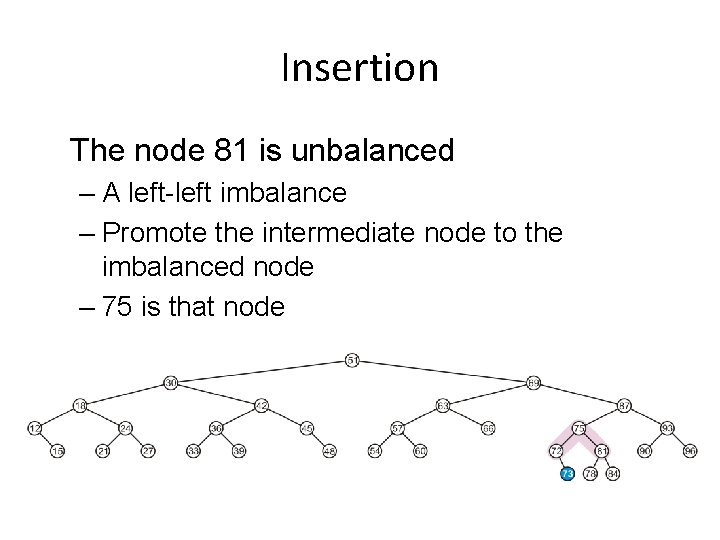
Insertion Insert 73

Insertion The node 81 is unbalanced – A left-left imbalance

Insertion The node 81 is unbalanced – A left-left imbalance

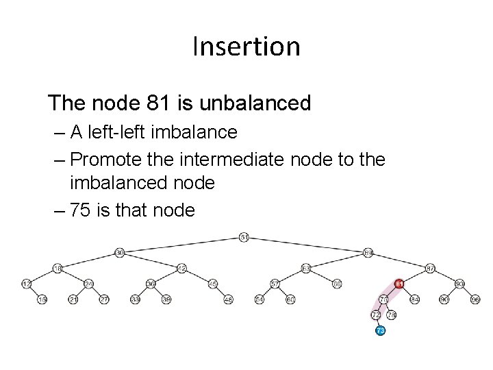
Insertion The node 81 is unbalanced – A left-left imbalance – Promote the intermediate node to the imbalanced node

Insertion The node 81 is unbalanced – A left-left imbalance – Promote the intermediate node to the imbalanced node – 75 is that node

Insertion The node 81 is unbalanced – A left-left imbalance – Promote the intermediate node to the imbalanced node – 75 is that node

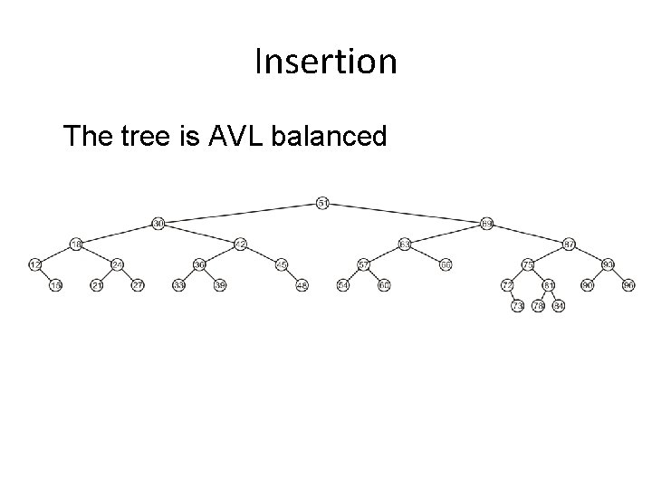
Insertion The tree is AVL balanced

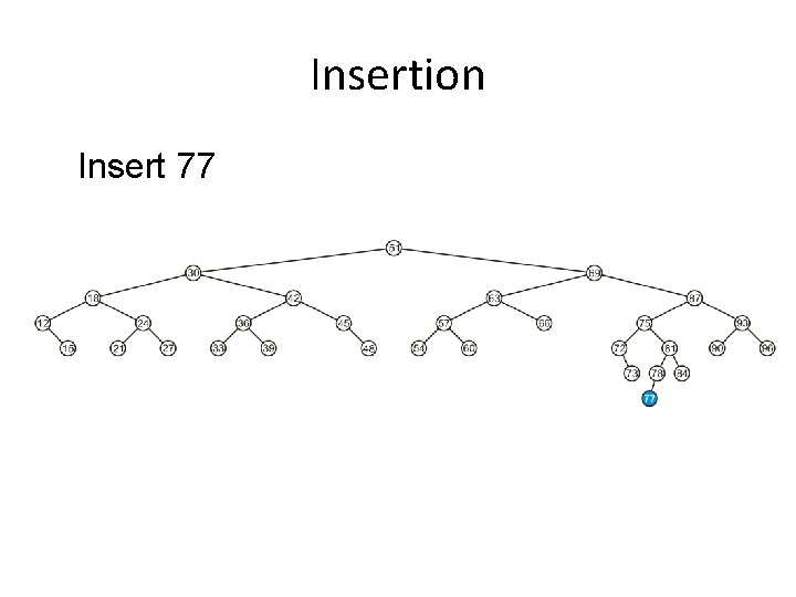
Insertion Insert 77

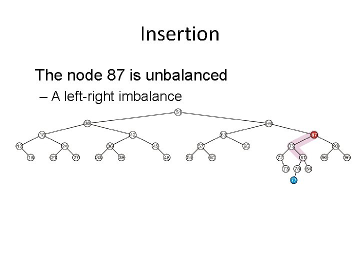
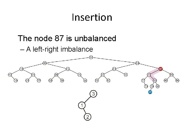
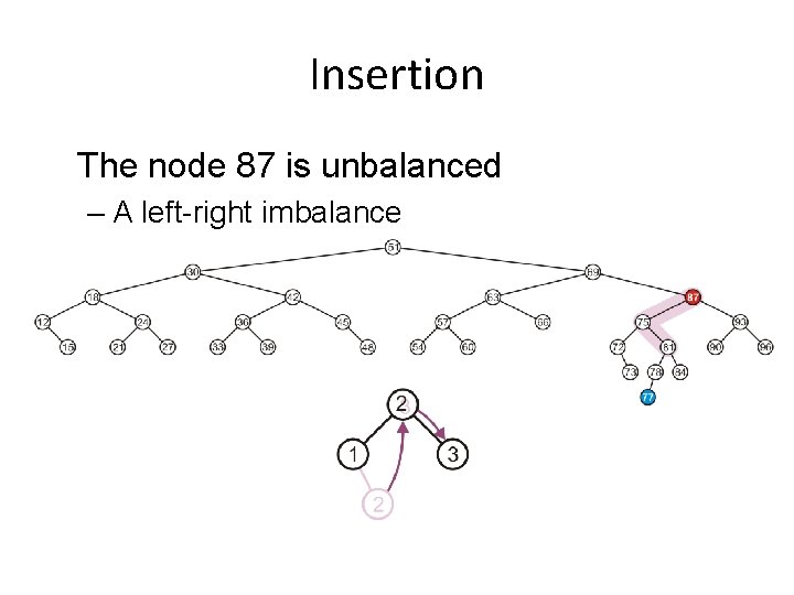
Insertion The node 87 is unbalanced – A left-right imbalance

Insertion The node 87 is unbalanced – A left-right imbalance

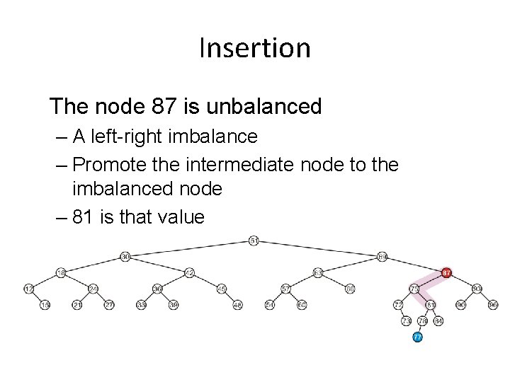
Insertion The node 87 is unbalanced – A left-right imbalance – Promote the intermediate node to the imbalanced node

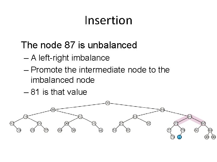
Insertion The node 87 is unbalanced – A left-right imbalance – Promote the intermediate node to the imbalanced node – 81 is that value

Insertion The node 87 is unbalanced – A left-right imbalance – Promote the intermediate node to the imbalanced node – 81 is that value

Insertion The tree is balanced

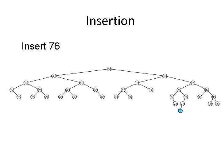
Insertion Insert 76

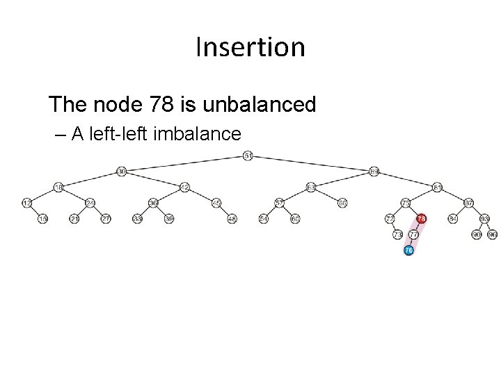
Insertion The node 78 is unbalanced – A left-left imbalance

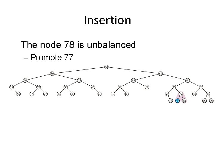
Insertion The node 78 is unbalanced – Promote 77

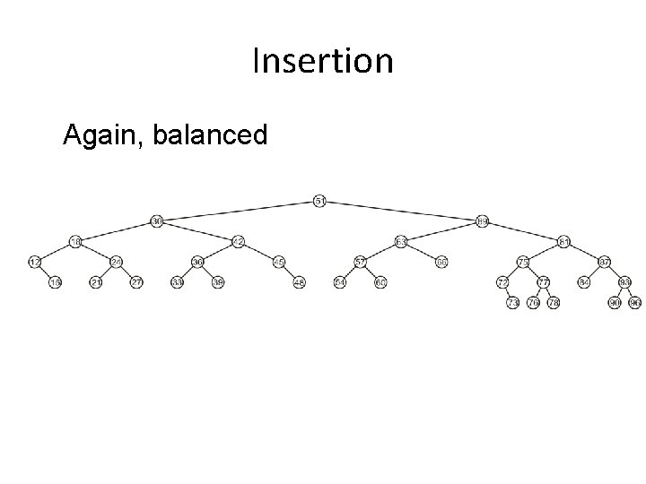
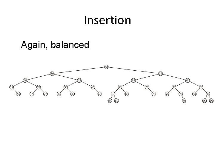
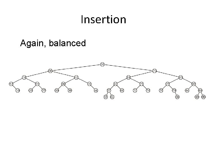
Insertion Again, balanced

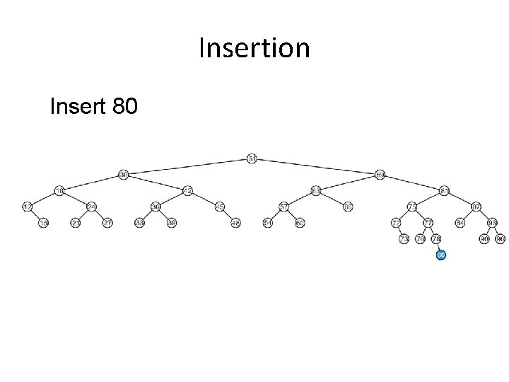
Insertion Insert 80

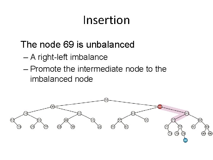
Insertion The node 69 is unbalanced – A right-left imbalance – Promote the intermediate node to the imbalanced node

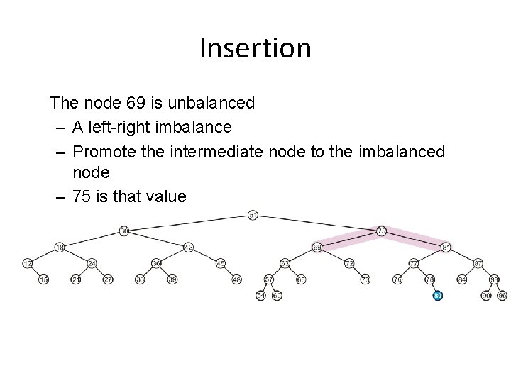
Insertion The node 69 is unbalanced – A left-right imbalance – Promote the intermediate node to the imbalanced node – 75 is that value

Insertion Again, balanced

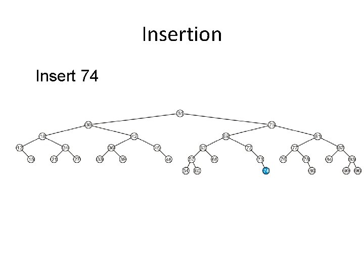
Insertion Insert 74

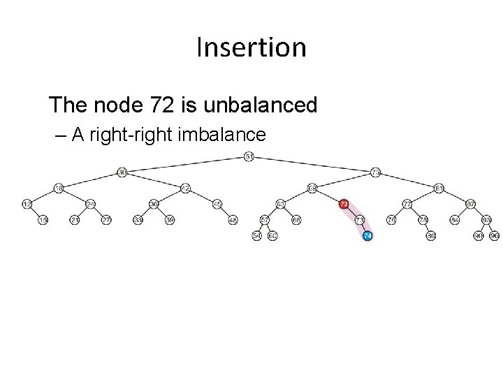
Insertion The node 72 is unbalanced – A right-right imbalance – Promote the intermediate node to the imbalanced node – 75 is that value

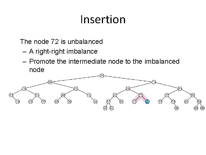
Insertion The node 72 is unbalanced – A right-right imbalance – Promote the intermediate node to the imbalanced node

Insertion Again, balanced

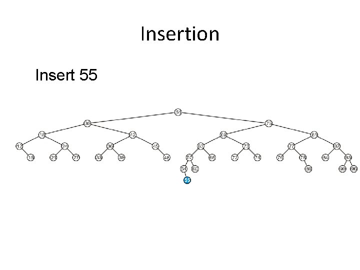
Insertion Insert 55

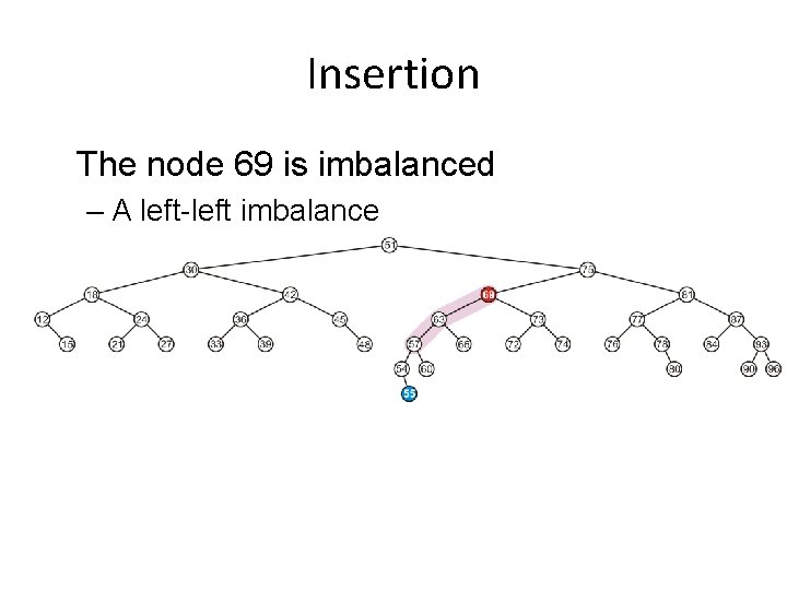
Insertion The node 69 is imbalanced – A left-left imbalance – Promote the intermediate node to the imbalanced node

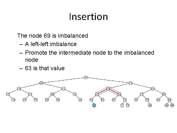
Insertion The node 69 is imbalanced – A left-left imbalance – Promote the intermediate node to the imbalanced node – 63 is that value

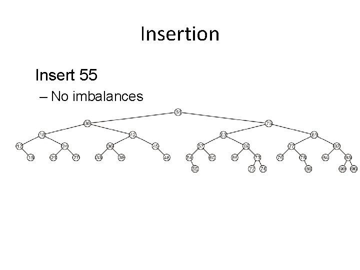
Insertion Insert 55 – No imbalances

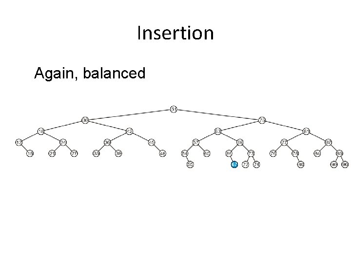
Insertion Again, balanced

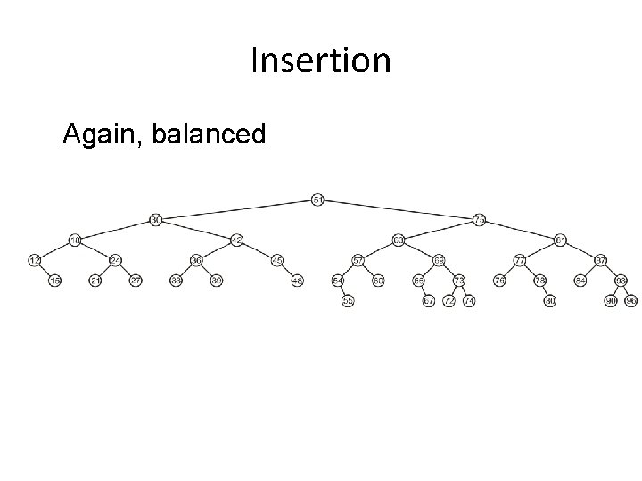
Insertion Again, balanced

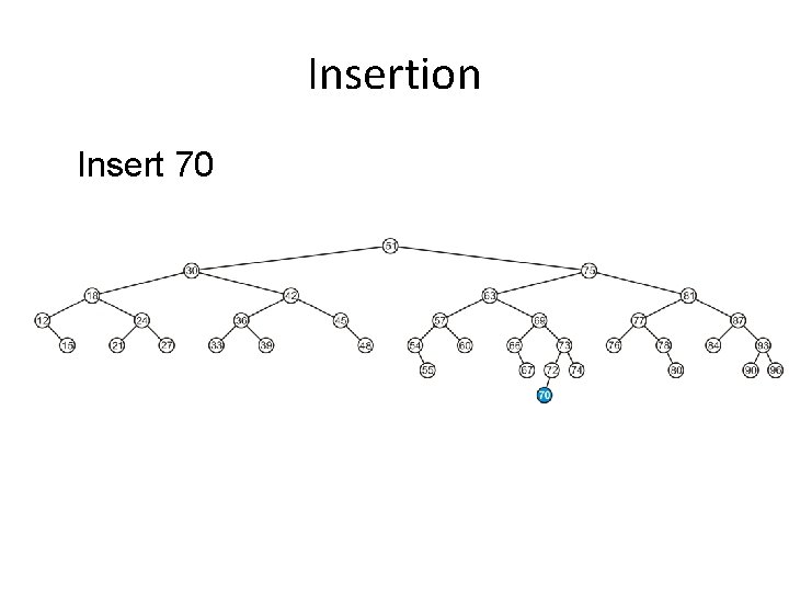
Insertion Insert 70

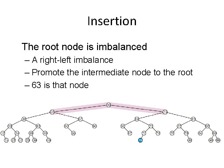
Insertion The root node is now imbalanced – A right-left imbalance – Promote the intermediate node to the root – 75 is that value

Insertion The root node is imbalanced – A right-left imbalance – Promote the intermediate node to the root – 63 is that node

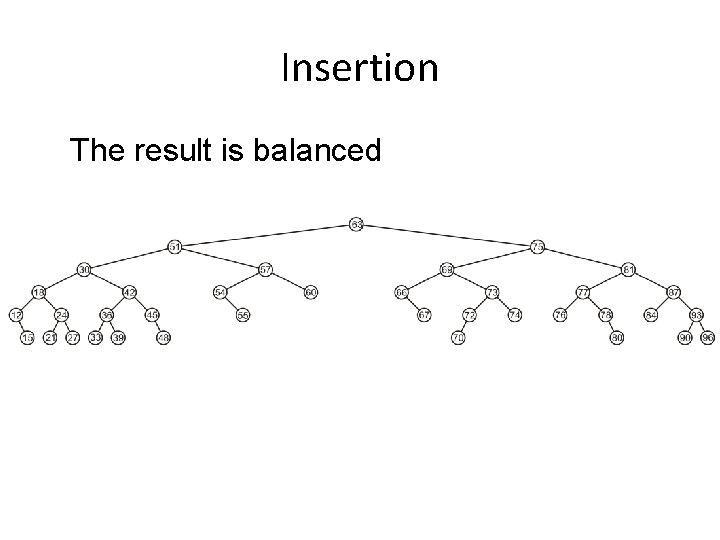
Insertion The result is balanced

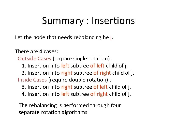
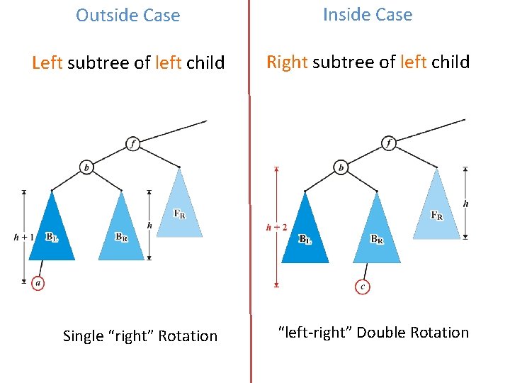
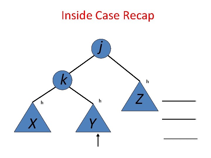
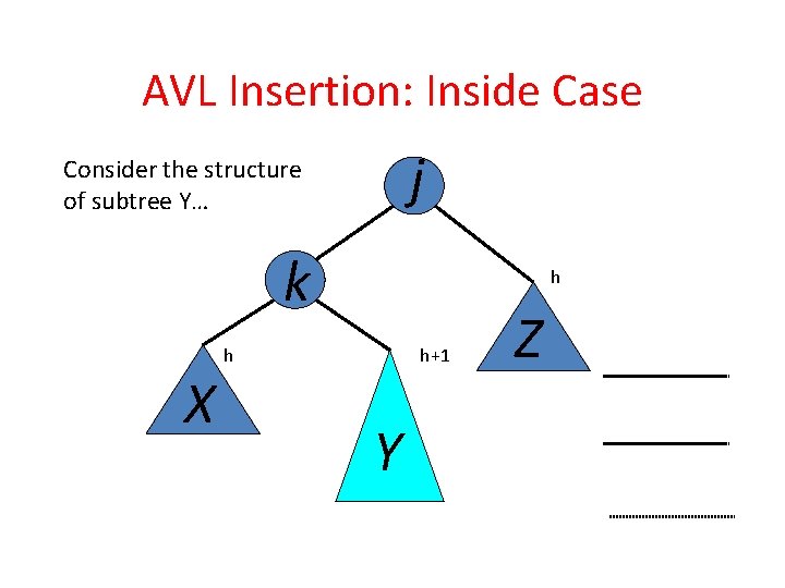
Summary : Insertions Let the node that needs rebalancing be j. There are 4 cases: Outside Cases (require single rotation) : 1. Insertion into left subtree of left child of j. 2. Insertion into right subtree of right child of j. Inside Cases (require double rotation) : 3. Insertion into right subtree of left child of j. 4. Insertion into left subtree of right child of j. The rebalancing is performed through four separate rotation algorithms.

Outside Case Inside Case Left subtree of left child Right subtree of left child Single “right” Rotation “left-right” Double Rotation

Inside Case Recap j k h h h X Y Z

AVL Insertion: Inside Case j Consider the structure of subtree Y… k X h h h+1 Y Z

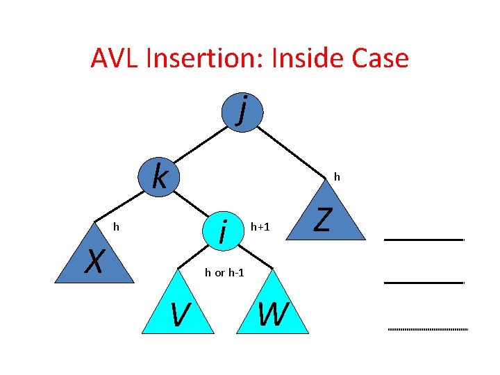
AVL Insertion: Inside Case j k h i h X h+1 h or h-1 V W Z

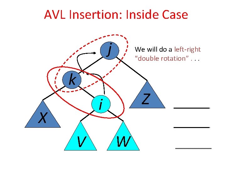
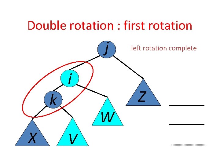
AVL Insertion: Inside Case j We will do a left-right “double rotation”. . . k Z i X V W

Double rotation : first rotation j i k X Z W V left rotation complete

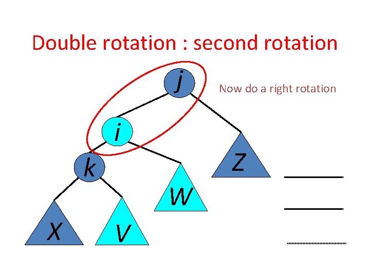
Double rotation : second rotation j i k X Z W V Now do a right rotation

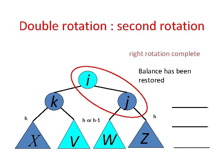
Double rotation : second rotation right rotation complete Balance has been restored i j k h h h or h-1 X V W Z

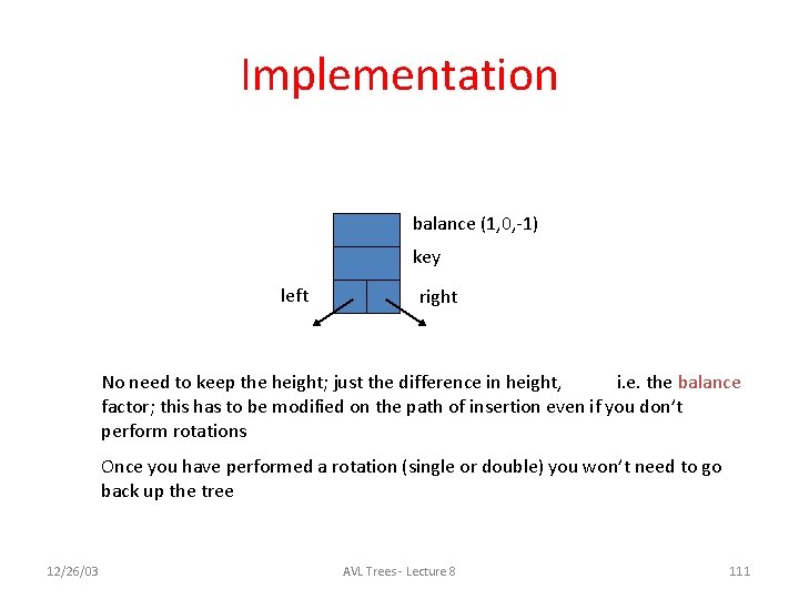
Implementation balance (1, 0, -1) key left right No need to keep the height; just the difference in height, i. e. the balance factor; this has to be modified on the path of insertion even if you don’t perform rotations Once you have performed a rotation (single or double) you won’t need to go back up the tree 12/26/03 AVL Trees - Lecture 8 111

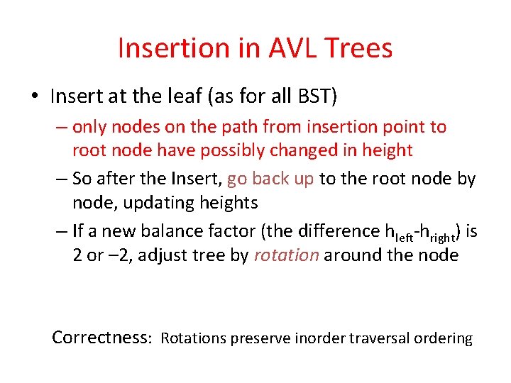
Insertion in AVL Trees • Insert at the leaf (as for all BST) – only nodes on the path from insertion point to root node have possibly changed in height – So after the Insert, go back up to the root node by node, updating heights – If a new balance factor (the difference hleft-hright) is 2 or – 2, adjust tree by rotation around the node Correctness: Rotations preserve inorder traversal ordering

Erase Removing a node from an AVL tree may cause more than one AVL imbalance – Like insert, erase must check after it has been successfully called on a child to see if it caused an imbalance – Unfortunately, it may cause multiple imbalances that must be corrected • Insertions will only cause one imbalance that must be fixed

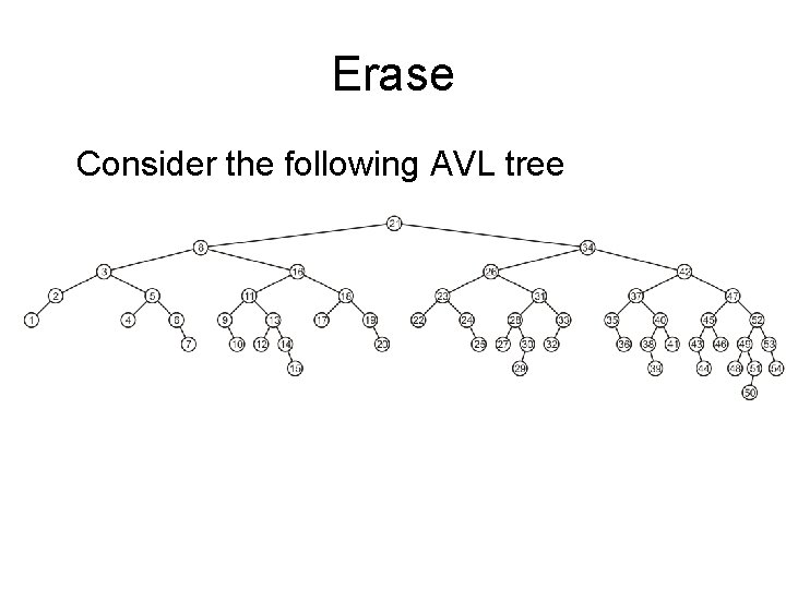
Erase Consider the following AVL tree

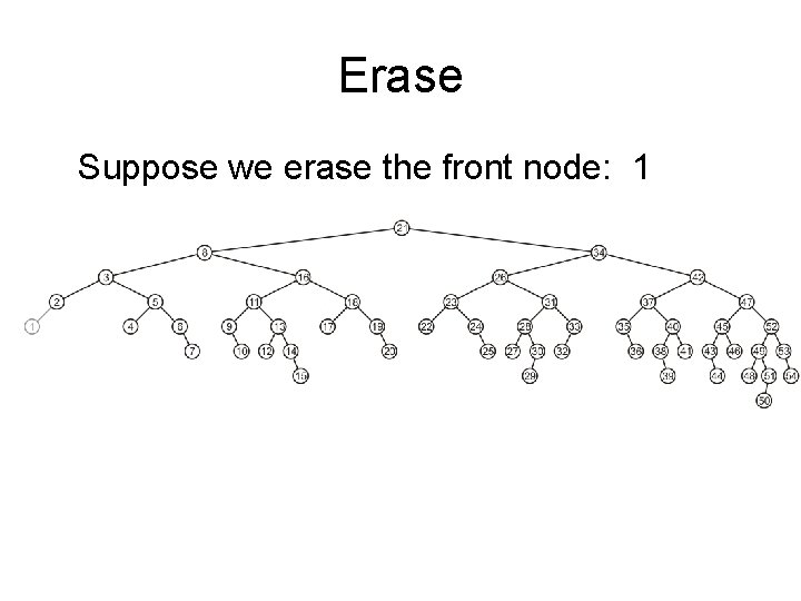
Erase Suppose we erase the front node: 1

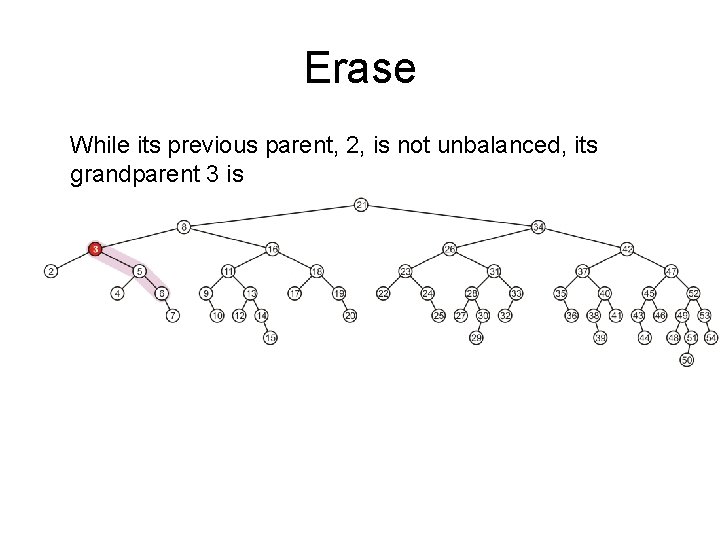
Erase While its previous parent, 2, is not unbalanced, its grandparent 3 is – The imbalance is in the right-right subtree

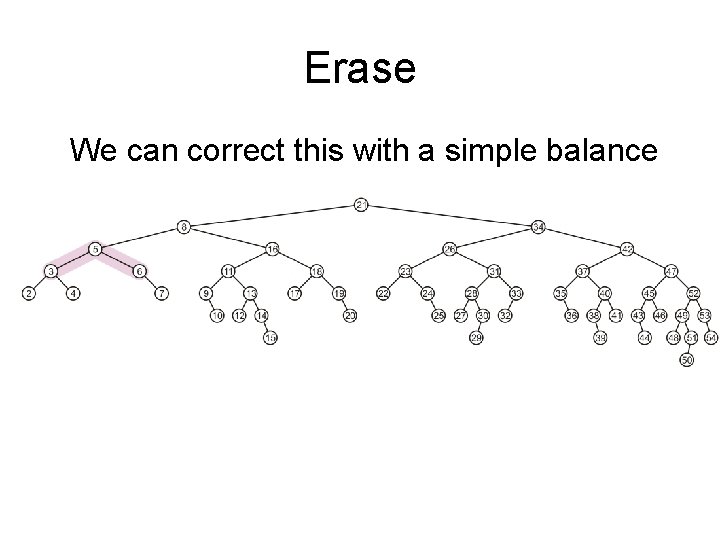
Erase We can correct this with a simple balance

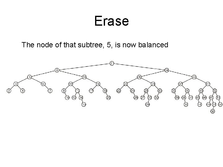
Erase The node of that subtree, 5, is now balanced

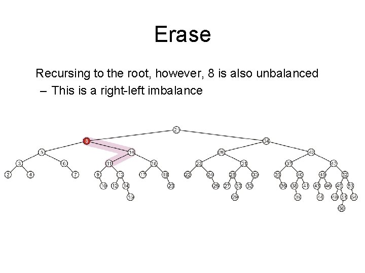
Erase Recursing to the root, however, 8 is also unbalanced – This is a right-left imbalance

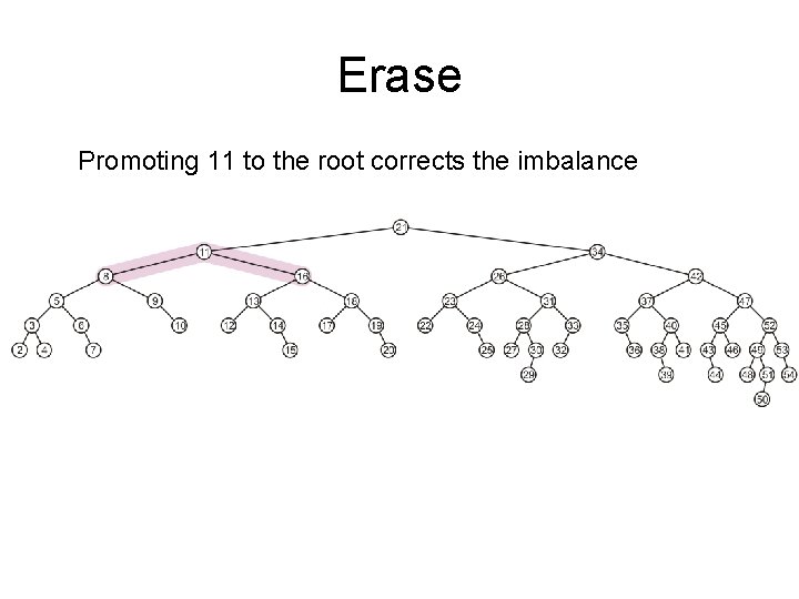
Erase Promoting 11 to the root corrects the imbalance

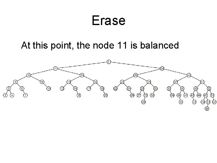
Erase At this point, the node 11 is balanced

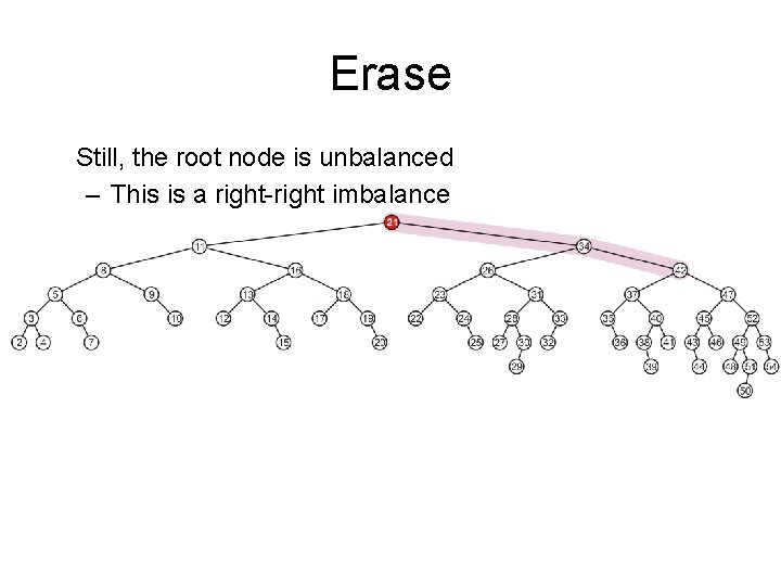
Erase Still, the root node is unbalanced – This is a right-right imbalance

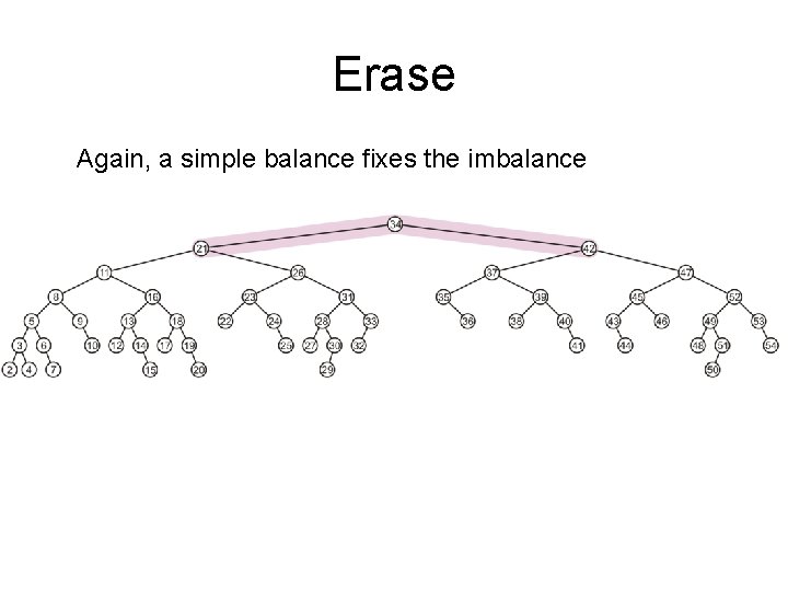
Erase Again, a simple balance fixes the imbalance

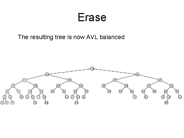
Erase The resulting tree is now AVL balanced

Pros and Cons of AVL Trees Arguments for AVL trees: 1. Search is O(log N) since AVL trees are always balanced. 2. Insertion and deletions are also O(logn) 3. The height balancing adds no more than a constant factor to the speed of insertion. Arguments against using AVL trees: 1. Difficult to program & debug; more space for balance factor. 2. Asymptotically faster but rebalancing costs time. 3. Most large searches are done in database systems on disk and use other structures (e. g. B-trees). 4. May be OK to have O(N) for a single operation if total run time for many consecutive operations is fast (e. g. Splay trees).