HASHING COL 106 Shweta Agrawal Amit Kumar Slide

HASHING COL 106 Shweta Agrawal, Amit Kumar Slide Courtesy : Linda Shapiro, Uwash Douglas W. Harder, UWaterloo

The Need for Speed • Data structures we have looked at so far – Use comparison operations to find items – Need O(log N) time for Find and Insert • In real world applications, N is typically between 100 and 100, 000 (or more) – log N is between 6. 6 and 16. 6 • Hash tables are an abstract data type designed for O(1) Find and Inserts 12/26/03 Hashing - Lecture 10 2

Fewer Functions Faster • compare lists and stacks – by reducing the flexibility of what we are allowed to do, we can increase the performance of the remaining operations – insert(L, X) into a list versus push(S, X) onto a stack • compare trees and hash tables – trees provide for known ordering of all elements – hash tables just let you (quickly) find an element 12/26/03 Hashing - Lecture 10 3

Limited Set of Hash Operations • For many applications, a limited set of operations is all that is needed – Insert, Find, and Delete – Note that no ordering of elements is implied • For example, a compiler needs to maintain information about the symbols in a program – user defined – language keywords Say that our data has format (key, value). How should we store it for efficient insert, find, delete?

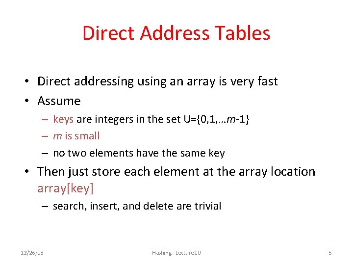
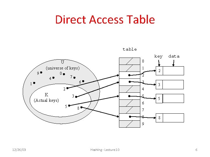
Direct Address Tables • Direct addressing using an array is very fast • Assume – keys are integers in the set U={0, 1, …m-1} – m is small – no two elements have the same key • Then just store each element at the array location array[key] – search, insert, and delete are trivial 12/26/03 Hashing - Lecture 10 5

Direct Access Table table key 0 U (universe of keys) 9 0 1 2 7 4 6 1 3 2 K (Actual keys) 4 3 5 data 5 6 8 2 3 5 7 8 8 9 12/26/03 Hashing - Lecture 10 6

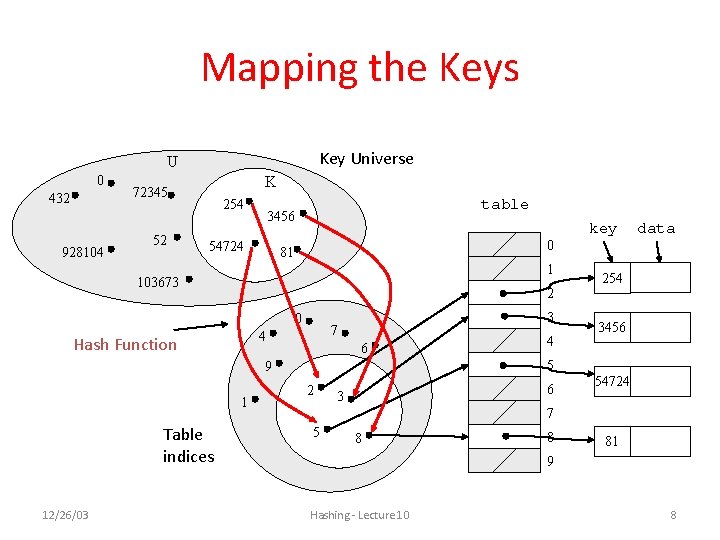
An Issue • If most keys in U are used – direct addressing can work very well (m small) • The largest possible key in U , say m, may be much larger than the number of elements actually stored (|U| much greater than |K|) – the table is very sparse and wastes space – in worst case, table too large to have in memory • If most keys in U are not used – need to map U to a smaller set closer in size to K 12/26/03 Hashing - Lecture 10 7

Mapping the Keys Key Universe U 0 432 928104 K 72345 52 254 table 3456 54724 key 0 81 1 103673 2 0 3 7 4 Hash Function 6 Table indices 12/26/03 4 254 3456 5 9 1 data 2 6 3 54724 7 5 8 8 81 9 Hashing - Lecture 10 8

Hashing Schemes • We want to store N items in a table of size M, at a location computed from the key K (which may not be numeric!) • Hash function – Method for computing table index from key • Need of a collision resolution strategy – How to handle two keys that hash to the same index 12/26/03 Hashing - Lecture 10 9

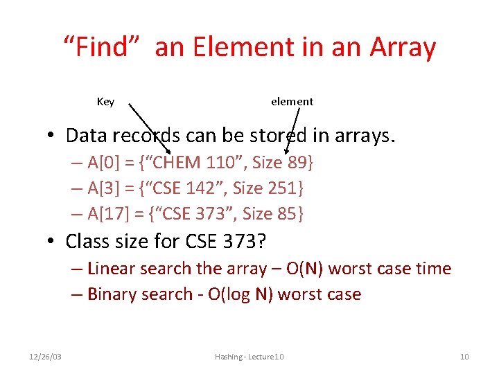
“Find” an Element in an Array Key element • Data records can be stored in arrays. – A[0] = {“CHEM 110”, Size 89} – A[3] = {“CSE 142”, Size 251} – A[17] = {“CSE 373”, Size 85} • Class size for CSE 373? – Linear search the array – O(N) worst case time – Binary search - O(log N) worst case 12/26/03 Hashing - Lecture 10 10

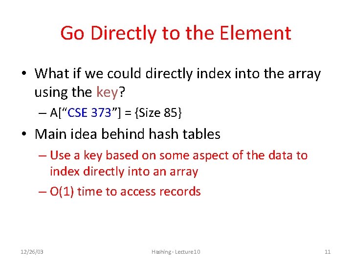
Go Directly to the Element • What if we could directly index into the array using the key? – A[“CSE 373”] = {Size 85} • Main idea behind hash tables – Use a key based on some aspect of the data to index directly into an array – O(1) time to access records 12/26/03 Hashing - Lecture 10 11

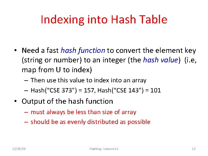
Indexing into Hash Table • Need a fast hash function to convert the element key (string or number) to an integer (the hash value) (i. e, map from U to index) – Then use this value to index into an array – Hash(“CSE 373”) = 157, Hash(“CSE 143”) = 101 • Output of the hash function – must always be less than size of array – should be as evenly distributed as possible 12/26/03 Hashing - Lecture 10 12

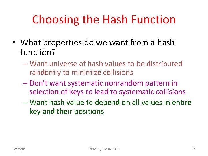
Choosing the Hash Function • What properties do we want from a hash function? – Want universe of hash values to be distributed randomly to minimize collisions – Don’t want systematic nonrandom pattern in selection of keys to lead to systematic collisions – Want hash value to depend on all values in entire key and their positions 12/26/03 Hashing - Lecture 10 13

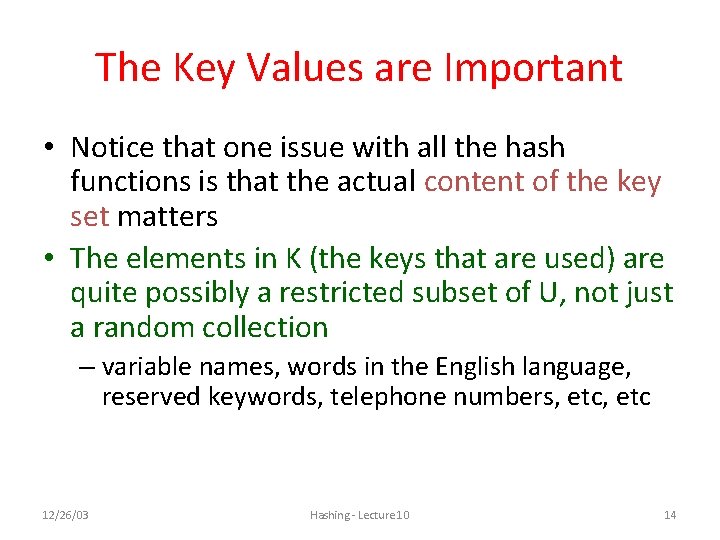
The Key Values are Important • Notice that one issue with all the hash functions is that the actual content of the key set matters • The elements in K (the keys that are used) are quite possibly a restricted subset of U, not just a random collection – variable names, words in the English language, reserved keywords, telephone numbers, etc 12/26/03 Hashing - Lecture 10 14

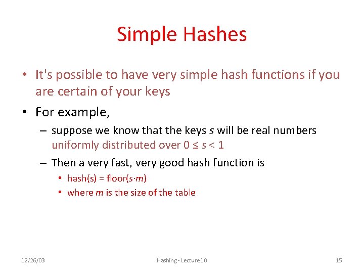
Simple Hashes • It's possible to have very simple hash functions if you are certain of your keys • For example, – suppose we know that the keys s will be real numbers uniformly distributed over 0 ≤ s < 1 – Then a very fast, very good hash function is • hash(s) = floor(s·m) • where m is the size of the table 12/26/03 Hashing - Lecture 10 15

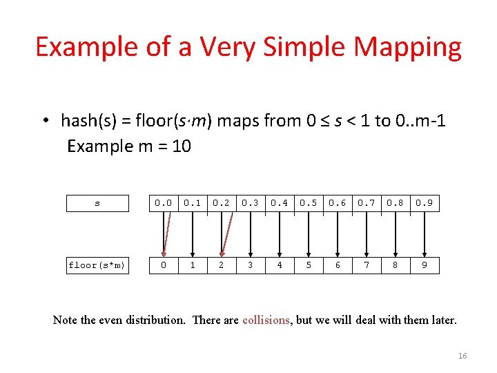
Example of a Very Simple Mapping • hash(s) = floor(s·m) maps from 0 ≤ s < 1 to 0. . m-1 Example m = 10 s 0. 0 0. 1 0. 2 0. 3 0. 4 0. 5 0. 6 0. 7 0. 8 0. 9 floor(s*m) 0 1 2 3 4 5 6 7 8 9 Note the even distribution. There are collisions, but we will deal with them later. 16

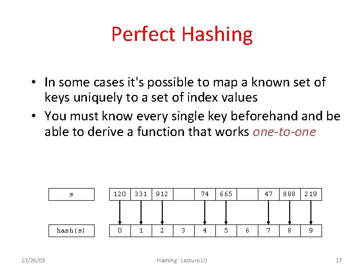
Perfect Hashing • In some cases it's possible to map a known set of keys uniquely to a set of index values • You must know every single key beforehand be able to derive a function that works one-to-one 12/26/03 s 120 331 912 hash(s) 0 1 2 3 74 665 4 5 Hashing - Lecture 10 6 47 888 219 7 8 9 17

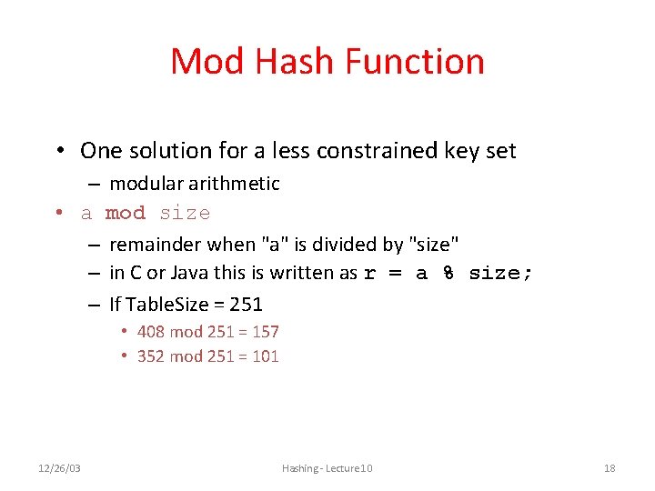
Mod Hash Function • One solution for a less constrained key set – modular arithmetic • a mod size – remainder when "a" is divided by "size" – in C or Java this is written as r = a % size; – If Table. Size = 251 • 408 mod 251 = 157 • 352 mod 251 = 101 12/26/03 Hashing - Lecture 10 18

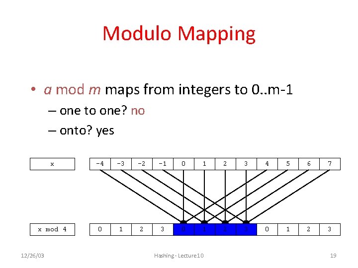
Modulo Mapping • a mod m maps from integers to 0. . m-1 – one to one? no – onto? yes x -4 -3 -2 -1 0 1 2 3 4 5 6 7 x mod 4 0 1 2 3 12/26/03 Hashing - Lecture 10 19

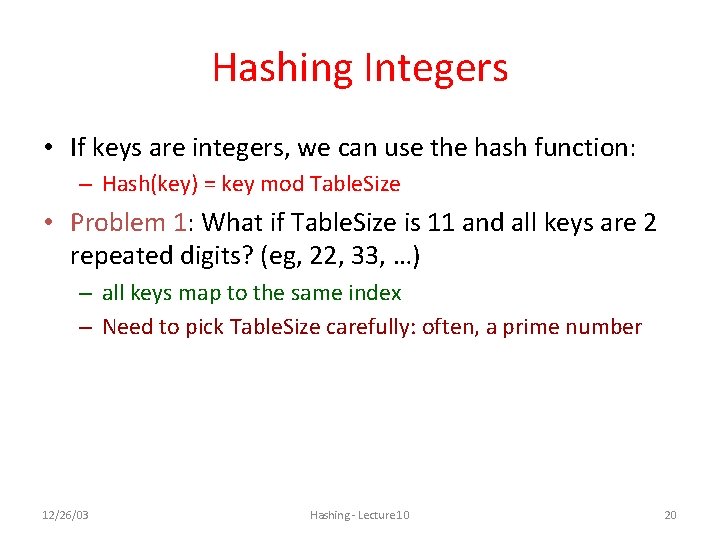
Hashing Integers • If keys are integers, we can use the hash function: – Hash(key) = key mod Table. Size • Problem 1: What if Table. Size is 11 and all keys are 2 repeated digits? (eg, 22, 33, …) – all keys map to the same index – Need to pick Table. Size carefully: often, a prime number 12/26/03 Hashing - Lecture 10 20

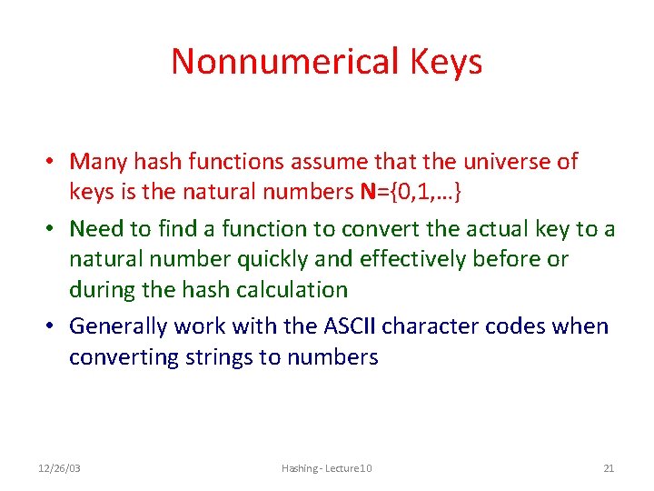
Nonnumerical Keys • Many hash functions assume that the universe of keys is the natural numbers N={0, 1, …} • Need to find a function to convert the actual key to a natural number quickly and effectively before or during the hash calculation • Generally work with the ASCII character codes when converting strings to numbers 12/26/03 Hashing - Lecture 10 21

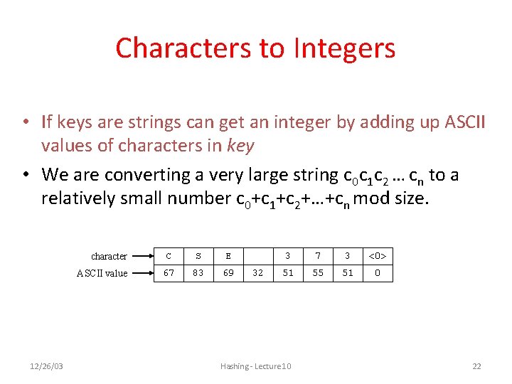
Characters to Integers • If keys are strings can get an integer by adding up ASCII values of characters in key • We are converting a very large string c 0 c 1 c 2 … cn to a relatively small number c 0+c 1+c 2+…+cn mod size. 12/26/03 character C S E ASCII value 67 83 69 32 3 7 3 <0> 51 55 51 0 Hashing - Lecture 10 22

Hash Must be Onto Table • Problem 2: What if Table. Size is 10, 000 and all keys are 8 or less characters long? – chars have values between 0 and 127 – Keys will hash only to positions 0 through 8*127 = 1016 • Need to distribute keys over the entire table or the extra space is wasted 12/26/03 Hashing - Lecture 10 23

Problems with Adding Characters • Problems with adding up character values for string keys – If string keys are short, will not hash evenly to all of the hash table – Different character combinations hash to same value • “abc”, “bca”, and “cab” all add up to the same value (recall this was Problem 1) 12/26/03 Hashing - Lecture 10 24

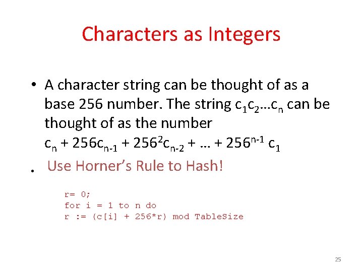
Characters as Integers • A character string can be thought of as a base 256 number. The string c 1 c 2…cn can be thought of as the number cn + 256 cn-1 + 2562 cn-2 + … + 256 n-1 c 1 • Use Horner’s Rule to Hash! r= 0; for i = 1 to n do r : = (c[i] + 256*r) mod Table. Size 25

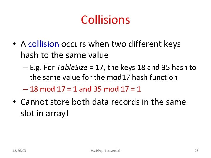
Collisions • A collision occurs when two different keys hash to the same value – E. g. For Table. Size = 17, the keys 18 and 35 hash to the same value for the mod 17 hash function – 18 mod 17 = 1 and 35 mod 17 = 1 • Cannot store both data records in the same slot in array! 12/26/03 Hashing - Lecture 10 26

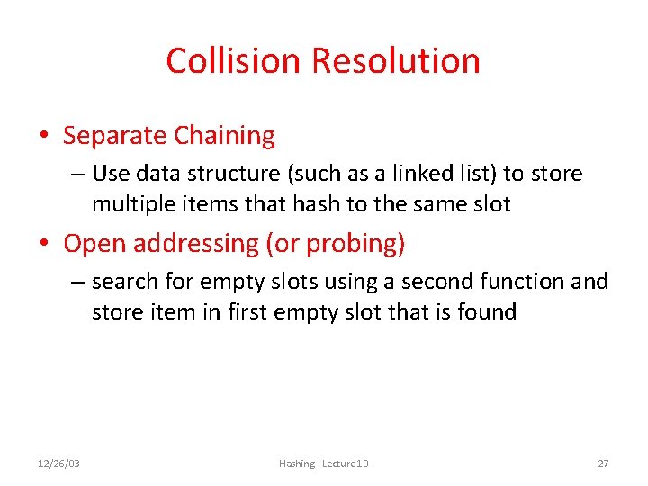
Collision Resolution • Separate Chaining – Use data structure (such as a linked list) to store multiple items that hash to the same slot • Open addressing (or probing) – search for empty slots using a second function and store item in first empty slot that is found 12/26/03 Hashing - Lecture 10 27

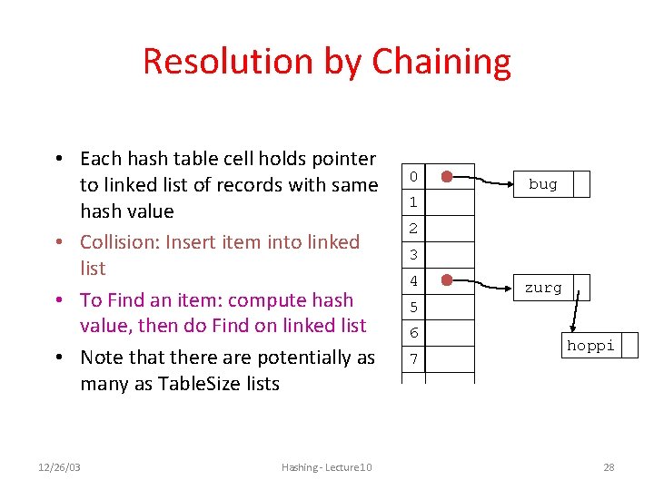
Resolution by Chaining • Each hash table cell holds pointer to linked list of records with same hash value • Collision: Insert item into linked list • To Find an item: compute hash value, then do Find on linked list • Note that there are potentially as many as Table. Size lists 12/26/03 Hashing - Lecture 10 0 1 bug 2 3 4 zurg 5 6 7 hoppi 28

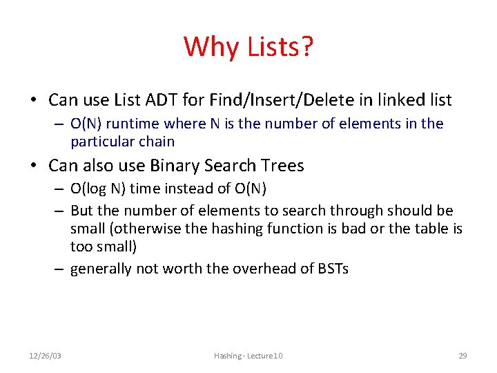
Why Lists? • Can use List ADT for Find/Insert/Delete in linked list – O(N) runtime where N is the number of elements in the particular chain • Can also use Binary Search Trees – O(log N) time instead of O(N) – But the number of elements to search through should be small (otherwise the hashing function is bad or the table is too small) – generally not worth the overhead of BSTs 12/26/03 Hashing - Lecture 10 29

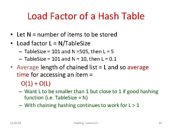
Load Factor of a Hash Table • Let N = number of items to be stored • Load factor L = N/Table. Size – Table. Size = 101 and N =505, then L = 5 – Table. Size = 101 and N = 10, then L = 0. 1 • Average length of chained list = L and so average time for accessing an item = O(1) + O(L) – Want L to be smaller than 1 but close to 1 if good hashing function (i. e. Table. Size ≈ N) – With chaining hashing continues to work for L > 1 12/26/03 Hashing - Lecture 10 30

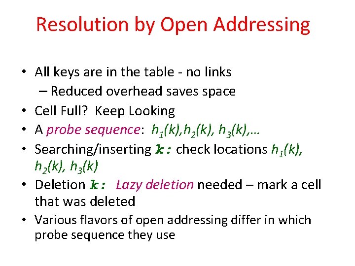
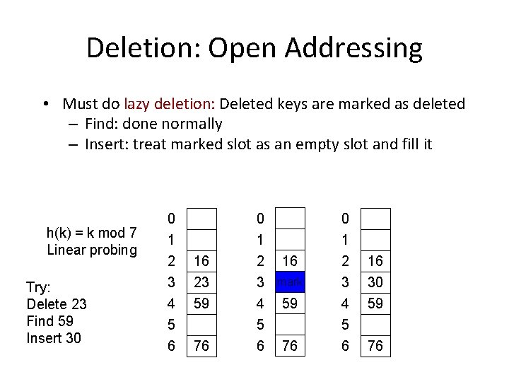
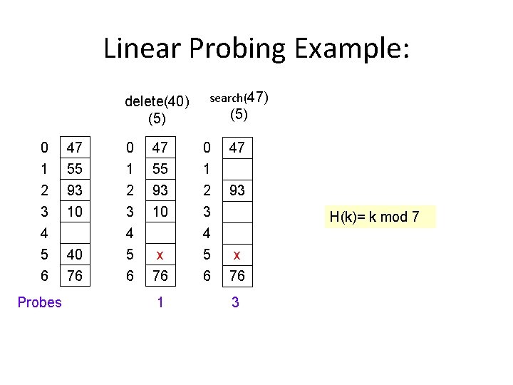
Resolution by Open Addressing • All keys are in the table - no links – Reduced overhead saves space • Cell Full? Keep Looking • A probe sequence: h 1(k), h 2(k), h 3(k), … • Searching/inserting k: check locations h 1(k), h 2(k), h 3(k) • Deletion k: Lazy deletion needed – mark a cell that was deleted • Various flavors of open addressing differ in which probe sequence they use

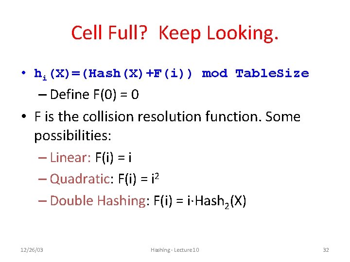
Cell Full? Keep Looking. • hi(X)=(Hash(X)+F(i)) mod Table. Size – Define F(0) = 0 • F is the collision resolution function. Some possibilities: – Linear: F(i) = i – Quadratic: F(i) = i 2 – Double Hashing: F(i) = i·Hash 2(X) 12/26/03 Hashing - Lecture 10 32

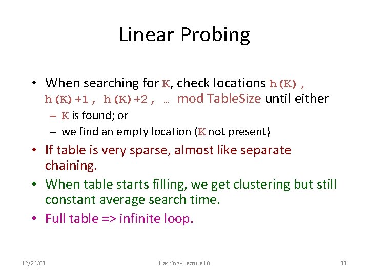
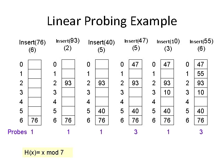
Linear Probing • When searching for K, check locations h(K), h(K)+1, h(K)+2, … mod Table. Size until either – K is found; or – we find an empty location (K not present) • If table is very sparse, almost like separate chaining. • When table starts filling, we get clustering but still constant average search time. • Full table => infinite loop. 12/26/03 Hashing - Lecture 10 33

Linear Probing Example Insert(76) (2) 0 1 2 3 4 5 6 Insert(93) 76 2 3 4 5 6 Probes 1 H(x)= x mod 7 0 1 93 2 93 3 4 76 1 Insert(47) Insert(40) (5) 5 6 (5) 1 Insert(55) (3) (6) 0 1 47 55 2 93 3 4 10 93 10 5 6 40 76 2 3 4 5 6 3 4 40 76 Insert(10) 5 6 40 76 3 1 40 76 3

Deletion: Open Addressing • Must do lazy deletion: Deleted keys are marked as deleted – Find: done normally – Insert: treat marked slot as an empty slot and fill it h(k) = k mod 7 Linear probing Try: Delete 23 Find 59 Insert 30 0 1 2 3 4 5 6 16 23 59 76 0 1 2 3 4 5 6 16 mark 59 76 0 1 2 3 4 5 6 16 30 59 76

Linear Probing Example: delete(40) (5) search(47) (5) 0 1 47 55 0 1 47 2 93 93 10 2 3 4 5 6 40 76 2 3 4 5 6 x 76 5 6 Probes 1 3 4 H(k)= k mod 7 x 76 3

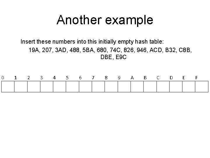
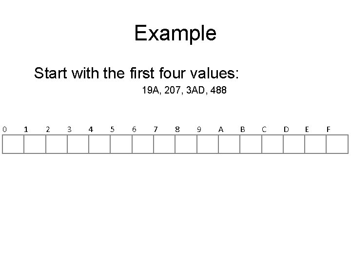
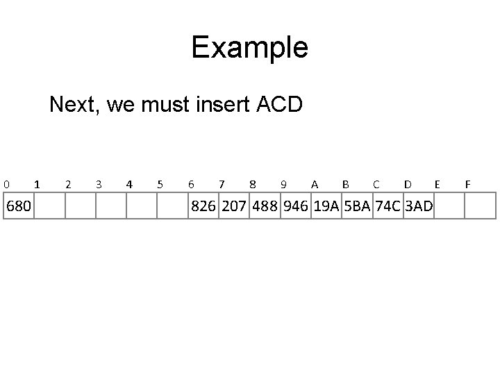
Another example Insert these numbers into this initially empty hash table: 19 A, 207, 3 AD, 488, 5 BA, 680, 74 C, 826, 946, ACD, B 32, C 8 B, DBE, E 9 C 0 1 2 3 4 5 6 7 8 9 A B C D E F

Example Start with the first four values: 19 A, 207, 3 AD, 488 0 1 2 3 4 5 6 7 8 9 A B C D E F

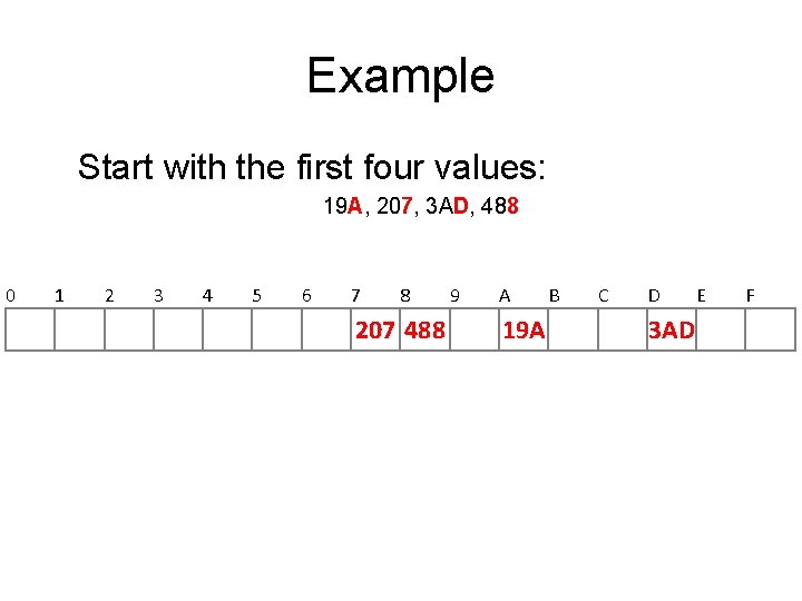
Example Start with the first four values: 19 A, 207, 3 AD, 488 0 1 2 3 4 5 6 7 8 207 488 9 A 19 A B C D 3 AD E F

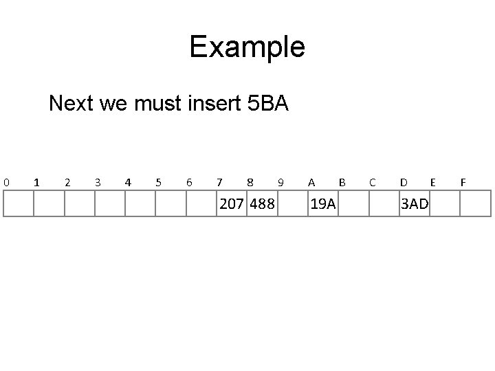
Example Next we must insert 5 BA 0 1 2 3 4 5 6 7 8 207 488 9 A 19 A B C D 3 AD E F

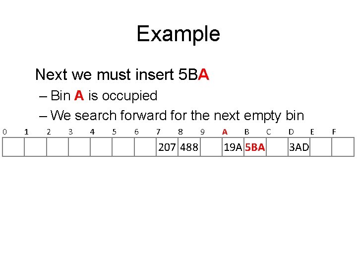
Example Next we must insert 5 BA – Bin A is occupied – We search forward for the next empty bin 0 1 2 3 4 5 6 7 8 207 488 9 A B 19 A 5 BA C D 3 AD E F

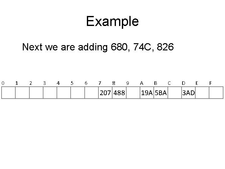
Example Next we are adding 680, 74 C, 826 0 1 2 3 4 5 6 7 8 207 488 9 A B 19 A 5 BA C D 3 AD E F

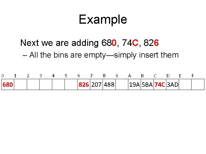
Example Next we are adding 680, 74 C, 826 – All the bins are empty—simply insert them 0 680 1 2 3 4 5 6 7 8 826 207 488 9 A B C D 19 A 5 BA 74 C 3 AD E F

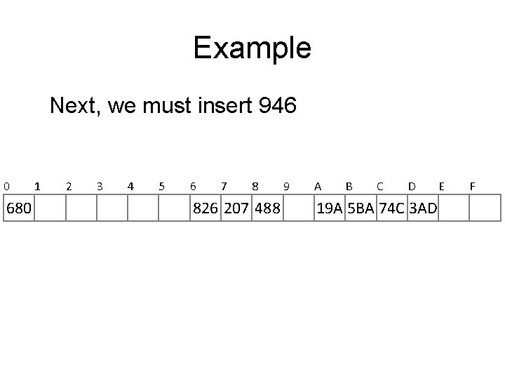
Example Next, we must insert 946 0 680 1 2 3 4 5 6 7 8 826 207 488 9 A B C D 19 A 5 BA 74 C 3 AD E F

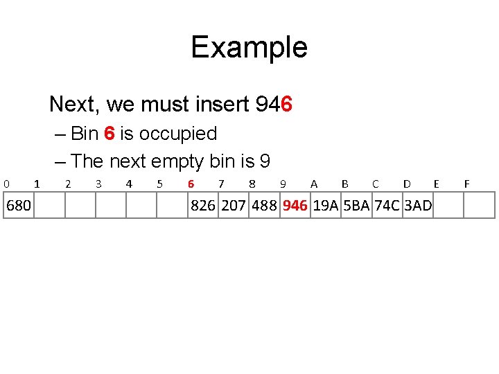
Example Next, we must insert 946 – Bin 6 is occupied – The next empty bin is 9 0 680 1 2 3 4 5 6 7 8 9 A B C D 826 207 488 946 19 A 5 BA 74 C 3 AD E F

Example Next, we must insert ACD 0 680 1 2 3 4 5 6 7 8 9 A B C D 826 207 488 946 19 A 5 BA 74 C 3 AD E F

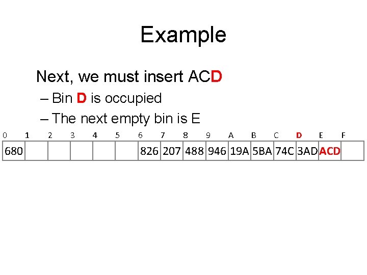
Example Next, we must insert ACD – Bin D is occupied – The next empty bin is E 0 680 1 2 3 4 5 6 7 8 9 A B C D E 826 207 488 946 19 A 5 BA 74 C 3 AD ACD F

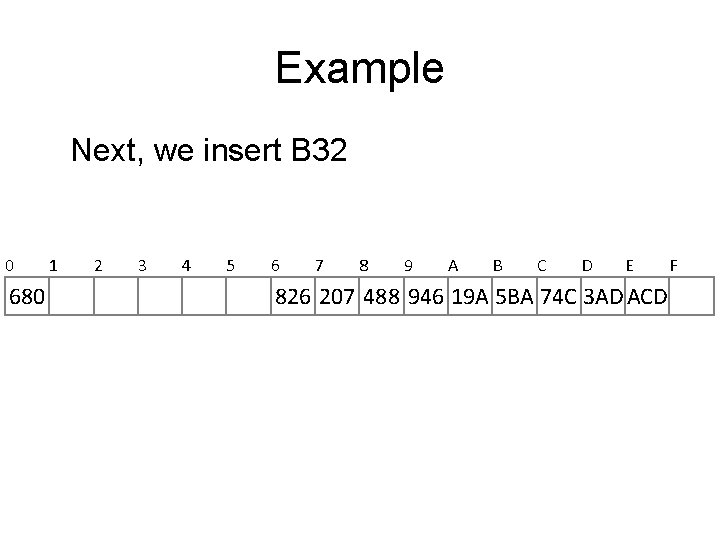
Example Next, we insert B 32 0 680 1 2 3 4 5 6 7 8 9 A B C D E 826 207 488 946 19 A 5 BA 74 C 3 AD ACD F

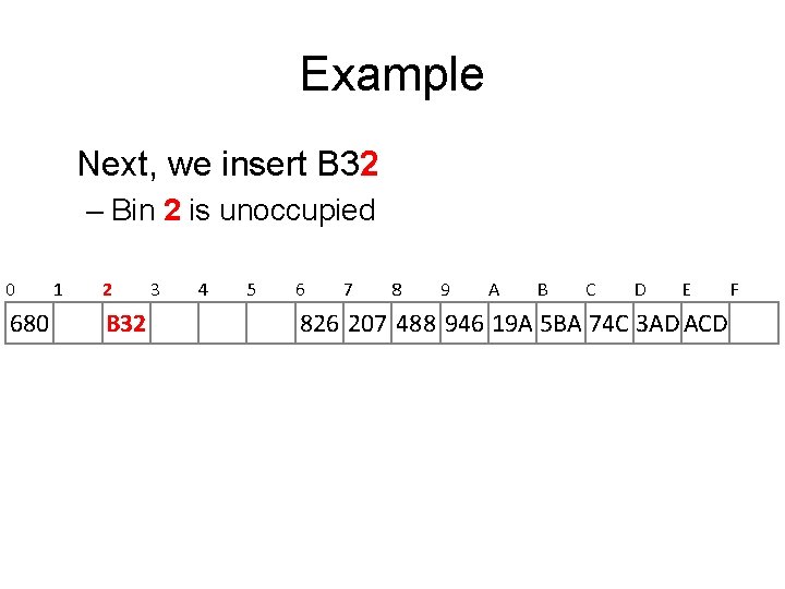
Example Next, we insert B 32 – Bin 2 is unoccupied 0 680 1 2 B 32 3 4 5 6 7 8 9 A B C D E 826 207 488 946 19 A 5 BA 74 C 3 AD ACD F

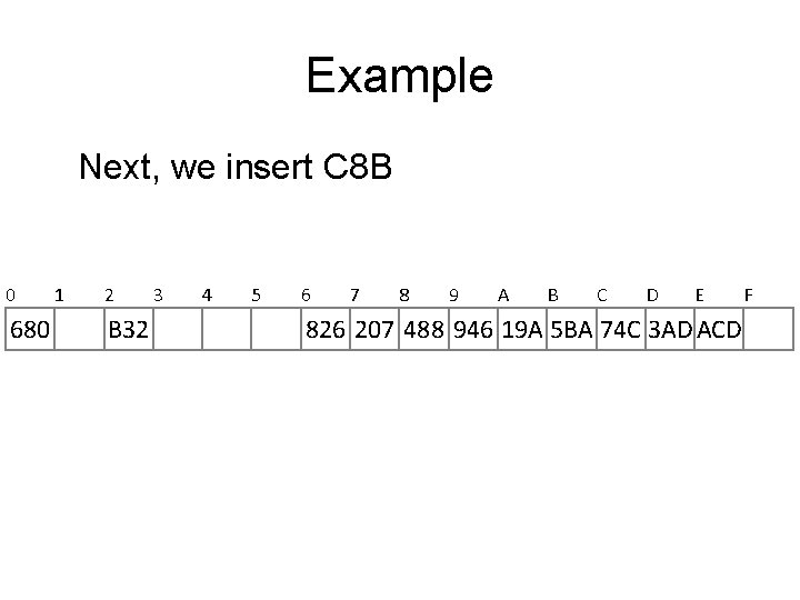
Example Next, we insert C 8 B 0 680 1 2 B 32 3 4 5 6 7 8 9 A B C D E 826 207 488 946 19 A 5 BA 74 C 3 AD ACD F

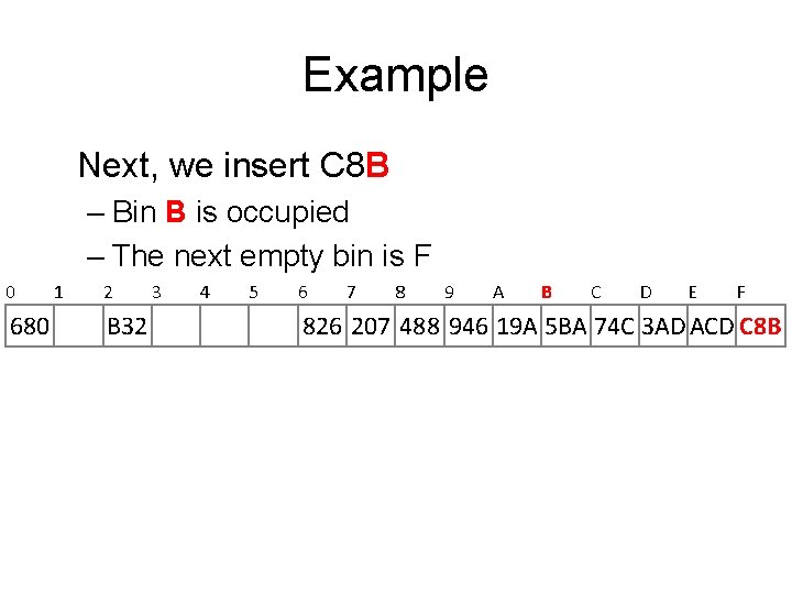
Example Next, we insert C 8 B – Bin B is occupied – The next empty bin is F 0 680 1 2 B 32 3 4 5 6 7 8 9 A B C D E F 826 207 488 946 19 A 5 BA 74 C 3 AD ACD C 8 B

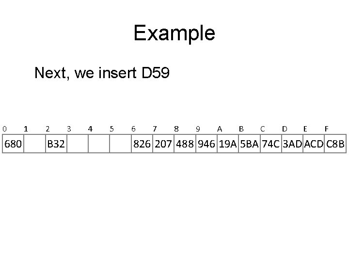
Example Next, we insert D 59 0 680 1 2 B 32 3 4 5 6 7 8 9 A B C D E F 826 207 488 946 19 A 5 BA 74 C 3 AD ACD C 8 B

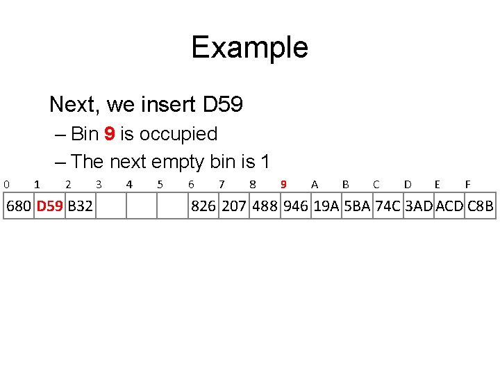
Example Next, we insert D 59 – Bin 9 is occupied – The next empty bin is 1 0 1 2 680 D 59 B 32 3 4 5 6 7 8 9 A B C D E F 826 207 488 946 19 A 5 BA 74 C 3 AD ACD C 8 B

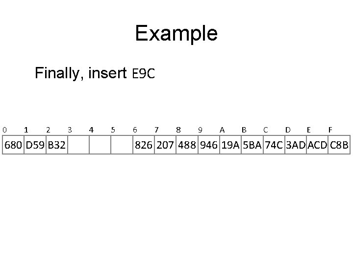
Example Finally, insert E 9 C 0 1 2 680 D 59 B 32 3 4 5 6 7 8 9 A B C D E F 826 207 488 946 19 A 5 BA 74 C 3 AD ACD C 8 B

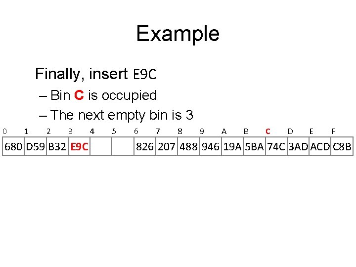
Example Finally, insert E 9 C – Bin C is occupied – The next empty bin is 3 0 1 2 3 680 D 59 B 32 E 9 C 4 5 6 7 8 9 A B C D E F 826 207 488 946 19 A 5 BA 74 C 3 AD ACD C 8 B

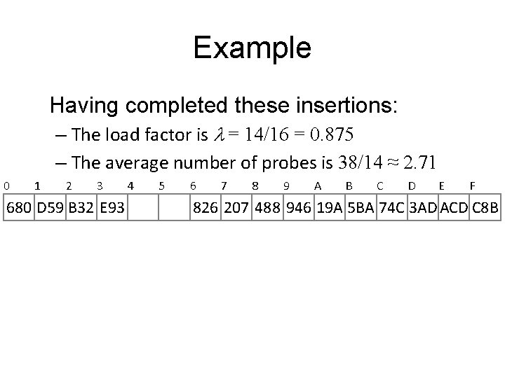
Example Having completed these insertions: – The load factor is l = 14/16 = 0. 875 – The average number of probes is 38/14 ≈ 2. 71 0 1 2 3 680 D 59 B 32 E 93 4 5 6 7 8 9 A B C D E F 826 207 488 946 19 A 5 BA 74 C 3 AD ACD C 8 B

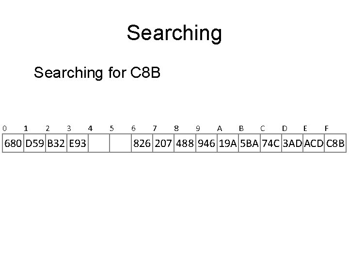
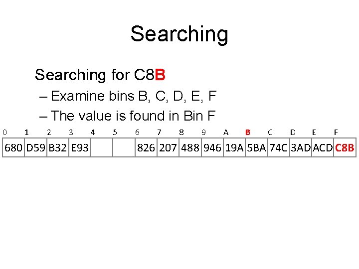
Searching for C 8 B 0 1 2 3 680 D 59 B 32 E 93 4 5 6 7 8 9 A B C D E F 826 207 488 946 19 A 5 BA 74 C 3 AD ACD C 8 B

Searching for C 8 B – Examine bins B, C, D, E, F – The value is found in Bin F 0 1 2 3 680 D 59 B 32 E 93 4 5 6 7 8 9 A B C D E F 826 207 488 946 19 A 5 BA 74 C 3 AD ACD C 8 B

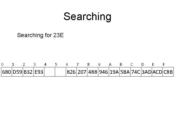
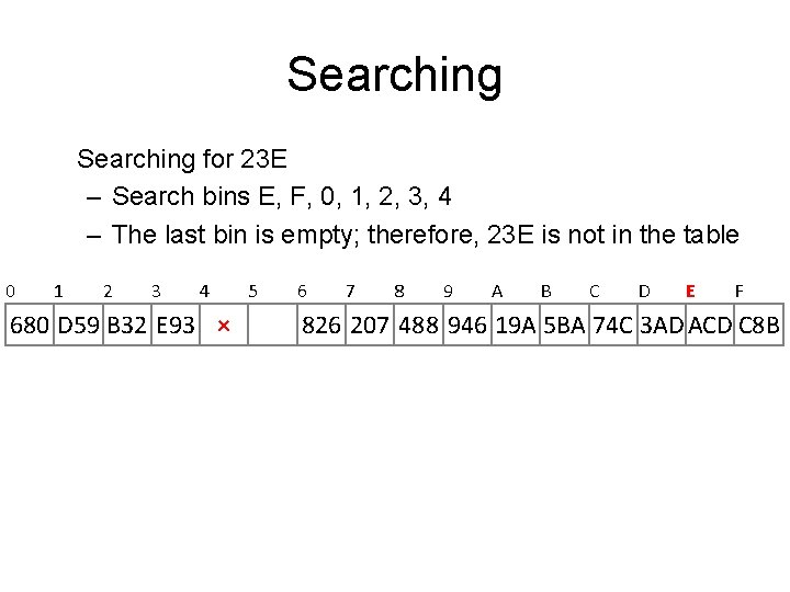
Searching for 23 E 0 1 2 3 680 D 59 B 32 E 93 4 5 6 7 8 9 A B C D E F 826 207 488 946 19 A 5 BA 74 C 3 AD ACD C 8 B

Searching for 23 E – Search bins E, F, 0, 1, 2, 3, 4 – The last bin is empty; therefore, 23 E is not in the table 0 1 2 3 4 680 D 59 B 32 E 93 × 5 6 7 8 9 A B C D E F 826 207 488 946 19 A 5 BA 74 C 3 AD ACD C 8 B

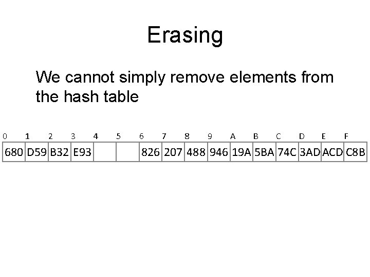
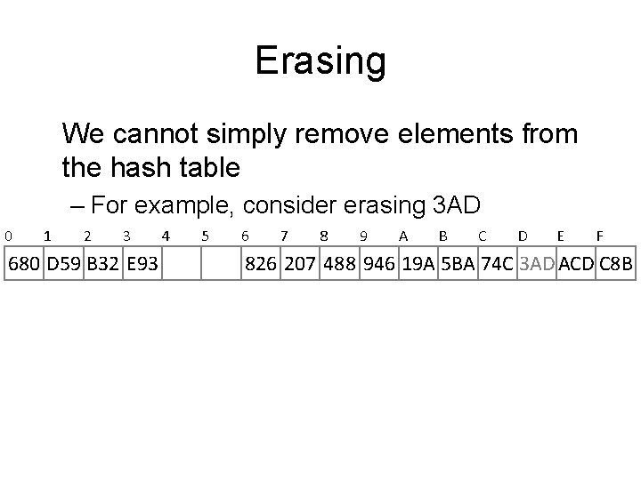
Erasing We cannot simply remove elements from the hash table 0 1 2 3 680 D 59 B 32 E 93 4 5 6 7 8 9 A B C D E F 826 207 488 946 19 A 5 BA 74 C 3 AD ACD C 8 B

Erasing We cannot simply remove elements from the hash table – For example, consider erasing 3 AD 0 1 2 3 680 D 59 B 32 E 93 4 5 6 7 8 9 A B C D E F 826 207 488 946 19 A 5 BA 74 C 3 AD ACD C 8 B

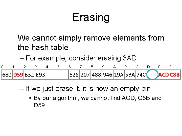
Erasing We cannot simply remove elements from the hash table – For example, consider erasing 3 AD 0 1 2 3 680 D 59 B 32 E 93 4 5 6 7 8 9 A B C D 826 207 488 946 19 A 5 BA 74 C E F ACD C 8 B – If we just erase it, it is now an empty bin • By our algorithm, we cannot find ACD, C 8 B and D 59

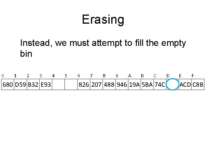
Erasing Instead, we must attempt to fill the empty bin 0 1 2 3 680 D 59 B 32 E 93 4 5 6 7 8 9 A B C 826 207 488 946 19 A 5 BA 74 C D E F ACD C 8 B

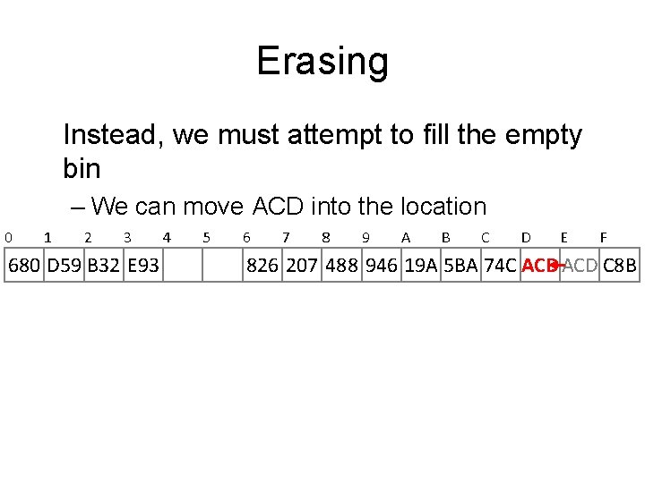
Erasing Instead, we must attempt to fill the empty bin – We can move ACD into the location 0 1 2 3 680 D 59 B 32 E 93 4 5 6 7 8 9 A B C D E F 826 207 488 946 19 A 5 BA 74 C ACD C 8 B

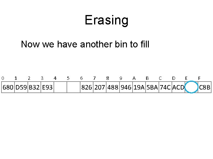
Erasing Now we have another bin to fill 0 1 2 3 680 D 59 B 32 E 93 4 5 6 7 8 9 A B C D 826 207 488 946 19 A 5 BA 74 C ACD E F C 8 B

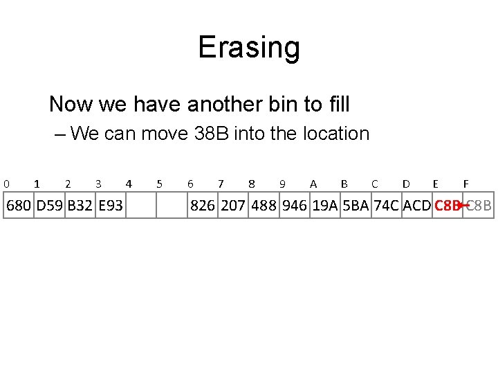
Erasing Now we have another bin to fill – We can move 38 B into the location 0 1 2 3 680 D 59 B 32 E 93 4 5 6 7 8 9 A B C D E F 826 207 488 946 19 A 5 BA 74 C ACD C 8 B

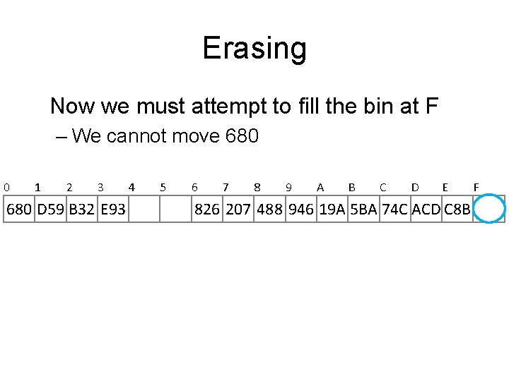
Erasing Now we must attempt to fill the bin at F – We cannot move 680 0 1 2 3 680 D 59 B 32 E 93 4 5 6 7 8 9 A B C D E 826 207 488 946 19 A 5 BA 74 C ACD C 8 B F

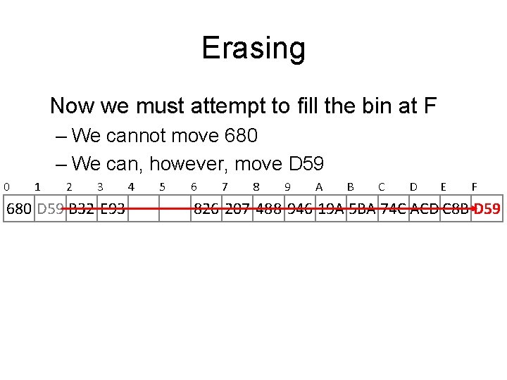
Erasing Now we must attempt to fill the bin at F – We cannot move 680 – We can, however, move D 59 0 1 2 3 680 D 59 B 32 E 93 4 5 6 7 8 9 A B C D E F 826 207 488 946 19 A 5 BA 74 C ACD C 8 B D 59

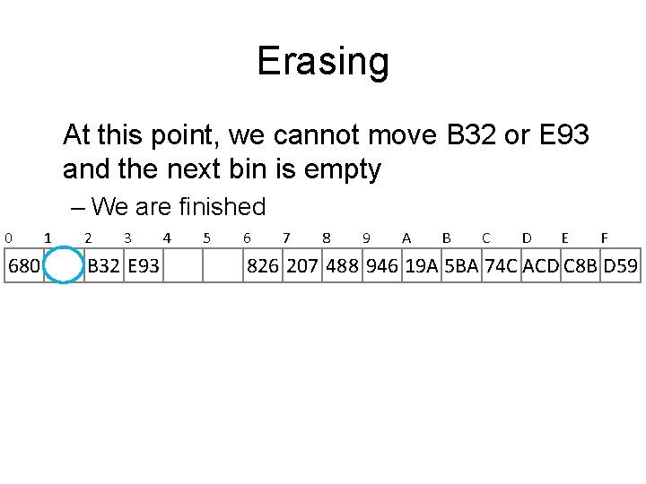
Erasing At this point, we cannot move B 32 or E 93 and the next bin is empty – We are finished 0 680 1 2 3 B 32 E 93 4 5 6 7 8 9 A B C D E F 826 207 488 946 19 A 5 BA 74 C ACD C 8 B D 59

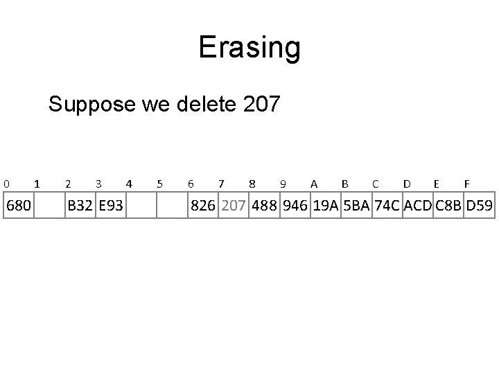
Erasing Suppose we delete 207 0 680 1 2 3 B 32 E 93 4 5 6 7 8 9 A B C D E F 826 207 488 946 19 A 5 BA 74 C ACD C 8 B D 59

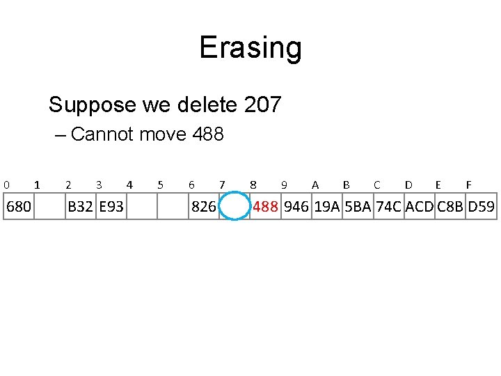
Erasing Suppose we delete 207 – Cannot move 488 0 680 1 2 3 B 32 E 93 4 5 6 826 7 8 9 A B C D E F 488 946 19 A 5 BA 74 C ACD C 8 B D 59

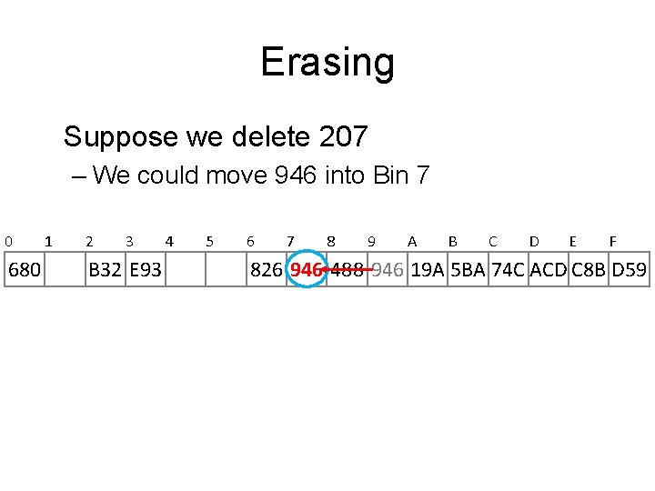
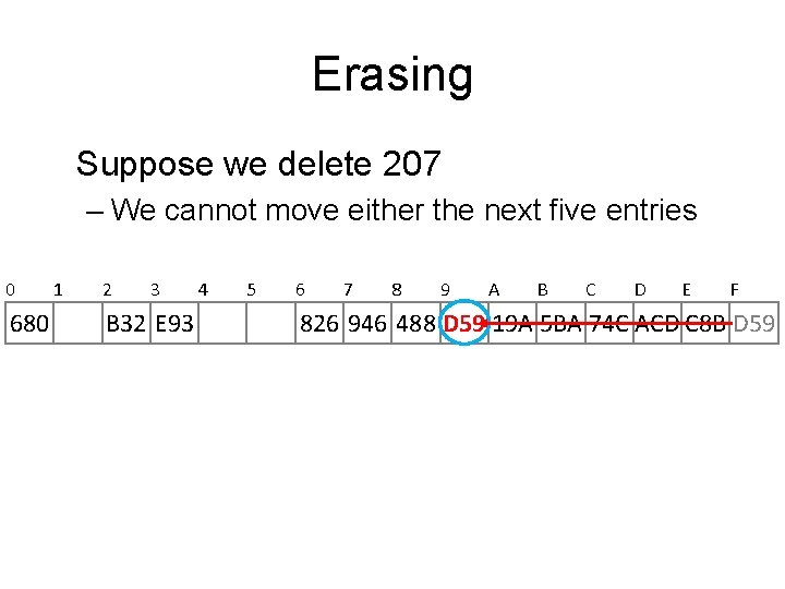
Erasing Suppose we delete 207 – We could move 946 into Bin 7 0 680 1 2 3 B 32 E 93 4 5 6 7 8 9 A B C D E F 826 946 488 946 19 A 5 BA 74 C ACD C 8 B D 59

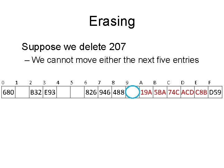
Erasing Suppose we delete 207 – We cannot move either the next five entries 0 680 1 2 3 B 32 E 93 4 5 6 7 8 826 946 488 9 A B C D E F 19 A 5 BA 74 C ACD C 8 B D 59

Erasing Suppose we delete 207 – We cannot move either the next five entries 0 680 1 2 3 B 32 E 93 4 5 6 7 8 9 A B C D E F 826 946 488 D 59 19 A 5 BA 74 C ACD C 8 B D 59

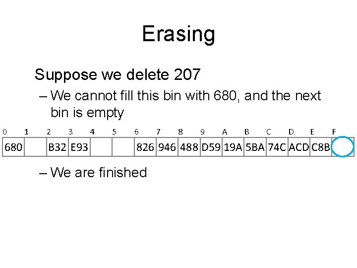
Erasing Suppose we delete 207 – We cannot fill this bin with 680, and the next bin is empty 0 680 1 2 3 B 32 E 93 4 5 6 7 8 9 A B C D E 826 946 488 D 59 19 A 5 BA 74 C ACD C 8 B – We are finished F

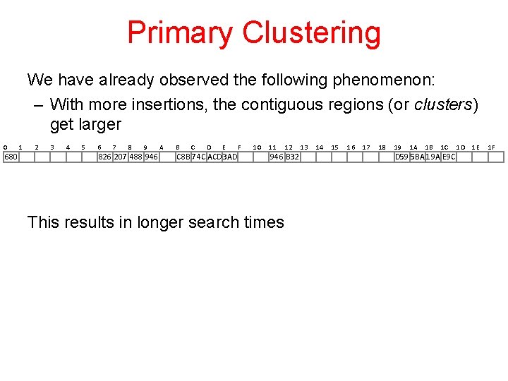
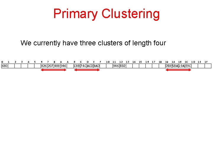
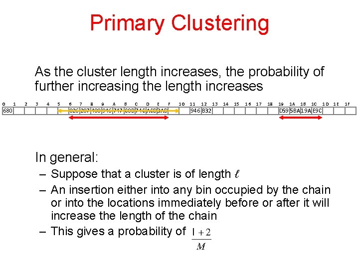
Primary Clustering We have already observed the following phenomenon: – With more insertions, the contiguous regions (or clusters) get larger 0 680 1 2 3 4 5 6 7 8 9 826 207 488 946 A B C D E C 8 B 74 C ACD 3 AD F 10 11 12 946 B 32 This results in longer search times 13 14 15 16 17 18 19 1 A 1 B 1 C D 59 5 BA 19 A E 9 C 1 D 1 E 1 F

Primary Clustering We currently have three clusters of length four 0 680 1 2 3 4 5 6 7 8 9 826 207 488 946 A B C D E C 8 B 74 C ACD 3 AD F 10 11 12 946 B 32 13 14 15 16 17 18 19 1 A 1 B 1 C D 59 5 BA 19 A E 9 C 1 D 1 E 1 F

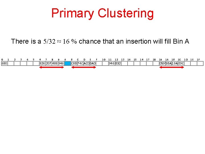
Primary Clustering There is a 5/32 ≈ 16 % chance that an insertion will fill Bin A 0 680 1 2 3 4 5 6 7 8 9 826 207 488 946 A B C D E C 8 B 74 C ACD 3 AD F 10 11 12 946 B 32 13 14 15 16 17 18 19 1 A 1 B 1 C D 59 5 BA 19 A E 9 C 1 D 1 E 1 F

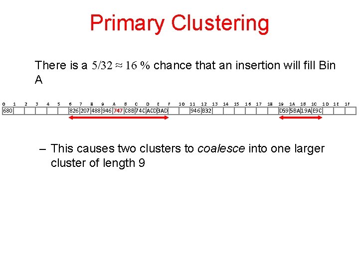
Primary Clustering There is a 5/32 ≈ 16 % chance that an insertion will fill Bin A 0 680 1 2 3 4 5 6 7 8 9 A B C D E 826 207 488 946 747 C 8 B 74 C ACD 3 AD F 10 11 12 946 B 32 13 14 15 16 17 18 19 1 A 1 B 1 C 1 D 1 E D 59 5 BA 19 A E 9 C – This causes two clusters to coalesce into one larger cluster of length 9 1 F

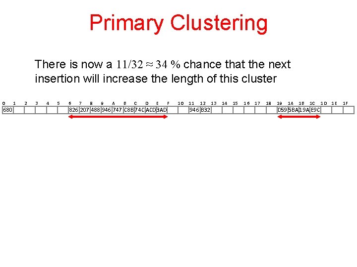
Primary Clustering There is now a 11/32 ≈ 34 % chance that the next insertion will increase the length of this cluster 0 680 1 2 3 4 5 6 7 8 9 A B C D E 826 207 488 946 747 C 8 B 74 C ACD 3 AD F 10 11 12 946 B 32 13 14 15 16 17 18 19 1 A 1 B 1 C D 59 5 BA 19 A E 9 C 1 D 1 E 1 F

Primary Clustering As the cluster length increases, the probability of further increasing the length increases 0 680 1 2 3 4 5 6 7 8 9 A B C D E 826 207 488 946 747 C 8 B 74 C ACD 3 AD F 10 11 12 946 B 32 13 14 15 16 17 18 19 1 A 1 B 1 C 1 D 1 E D 59 5 BA 19 A E 9 C In general: – Suppose that a cluster is of length ℓ – An insertion either into any bin occupied by the chain or into the locations immediately before or after it will increase the length of the chain – This gives a probability of 1 F

Quadratic Probing • When searching for X, check locations h 1(X), h 1(X)+ 12, h 1(X)+22, … mod Table. Size until either – X is found; or – we find an empty location (X not present) 12/26/03 Hashing - Lecture 10 83

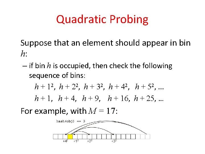
Quadratic Probing Suppose that an element should appear in bin h: – if bin h is occupied, then check the following sequence of bins: h + 12, h + 22, h + 32, h + 42, h + 52, . . . h + 1, h + 4, h + 9, h + 16, h + 25, … For example, with M = 17:

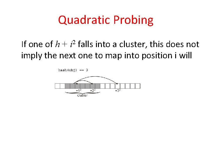
Quadratic Probing If one of h + i 2 falls into a cluster, this does not imply the next one to map into position i will

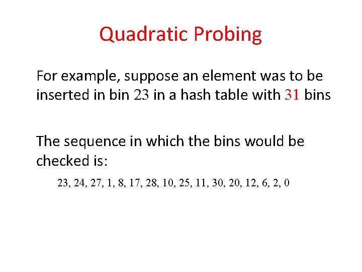
Quadratic Probing For example, suppose an element was to be inserted in bin 23 in a hash table with 31 bins The sequence in which the bins would be checked is: 23, 24, 27, 1, 8, 17, 28, 10, 25, 11, 30, 20, 12, 6, 2, 0

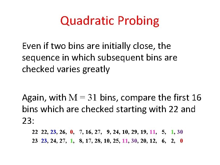
Quadratic Probing Even if two bins are initially close, the sequence in which subsequent bins are checked varies greatly Again, with M = 31 bins, compare the first 16 bins which are checked starting with 22 and 23: 22 22, 23, 26, 0, 7, 16, 27, 9, 24, 10, 29, 11, 5, 1, 30 23 23, 24, 27, 1, 8, 17, 28, 10, 25, 11, 30, 20, 12, 6, 2, 0

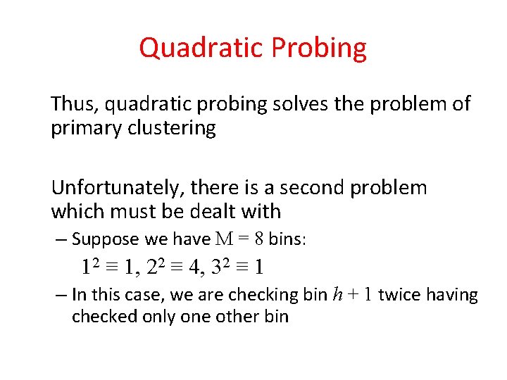
Quadratic Probing Thus, quadratic probing solves the problem of primary clustering Unfortunately, there is a second problem which must be dealt with – Suppose we have M = 8 bins: 12 ≡ 1, 22 ≡ 4, 32 ≡ 1 – In this case, we are checking bin h + 1 twice having checked only one other bin

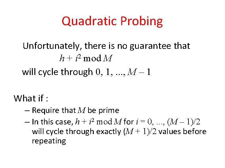
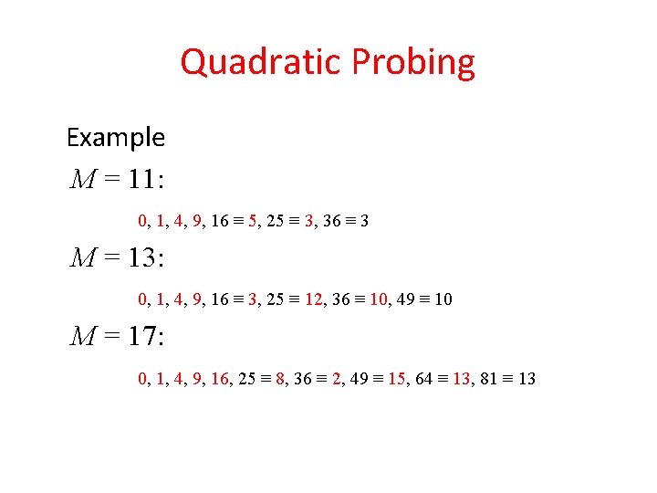
Quadratic Probing Unfortunately, there is no guarantee that h + i 2 mod M will cycle through 0, 1, . . . , M – 1 What if : – Require that M be prime – In this case, h + i 2 mod M for i = 0, . . . , (M – 1)/2 will cycle through exactly (M + 1)/2 values before repeating

Quadratic Probing Example M = 11: 0, 1, 4, 9, 16 ≡ 5, 25 ≡ 3, 36 ≡ 3 M = 13: 0, 1, 4, 9, 16 ≡ 3, 25 ≡ 12, 36 ≡ 10, 49 ≡ 10 M = 17: 0, 1, 4, 9, 16, 25 ≡ 8, 36 ≡ 2, 49 ≡ 15, 64 ≡ 13, 81 ≡ 13

Quadratic Probing Thus, quadratic probing avoids primary clustering – Unfortunately, we are not guaranteed that we will use all the bins In practice, if the hash function is reasonable, this is not a significant problem

Secondary Clustering The phenomenon of primary clustering does not occur with quadratic probing However, if multiple items all hash to the same initial bin, the same sequence of numbers will be followed – This is termed secondary clustering – The effect is less significant than that of primary clustering

Secondary Clustering Secondary clustering may be a problem if the hash function does not produce an even distribution of entries One solution to secondary is double hashing: associating with each element an initial bin (defined by one hash function) and a skip (defined by a second hash function)

Double Hashing • When searching for X, check locations h 1(X), h 1(X)+ h 2(X), h 1(X)+2*h 2(X), … mod Tablesize until either – X is found; or – we find an empty location (X not present) • Must be careful about h 2(X) – Not 0 and not a divisor of M – eg, h 1(k) = k mod m 1, h 2(k)=1+(k mod m 2) where m 2 is slightly less than m 1 12/26/03 Hashing - Lecture 10 96

Rules of Thumb • Separate chaining is simple but wastes space… • Linear probing uses space better, is fast when tables are sparse • Double hashing is space efficient, fast (get initial hash and increment at the same time), needs careful implementation

Rehashing – Rebuild the Table • Need to use lazy deletion if we use probing (why? ) – Need to mark array slots as deleted after Delete – consequently, deleting doesn’t make the table any less full than it was before the delete • If table gets too full or if many deletions have occurred, running time gets too long and Inserts may fail

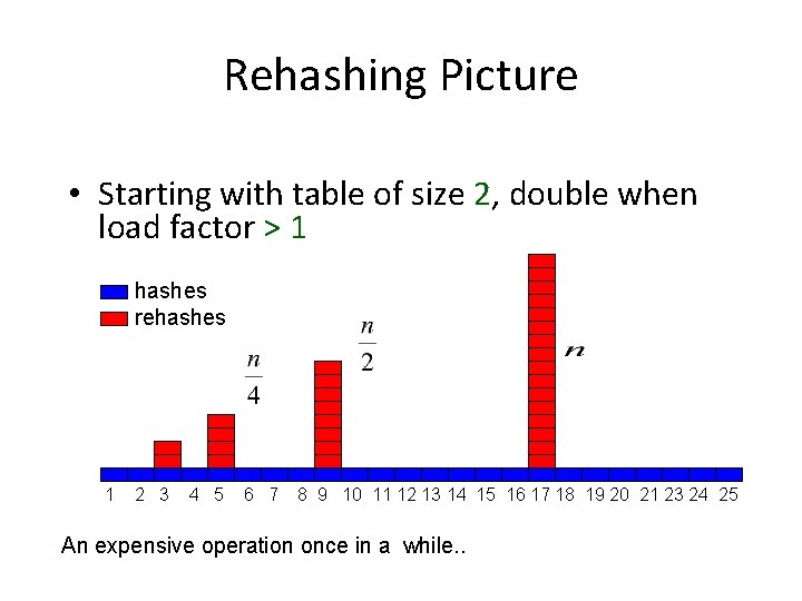
Rehashing • Build a bigger hash table of approximately twice the size when L exceeds a particular value – Go through old hash table, ignoring items marked deleted – Recompute hash value for each non-deleted key and put the item in new position in new table – Cannot just copy data from old table because the bigger table has a new hash function • Running time is O(N) but happens very infrequently – Not good for real-time safety critical applications

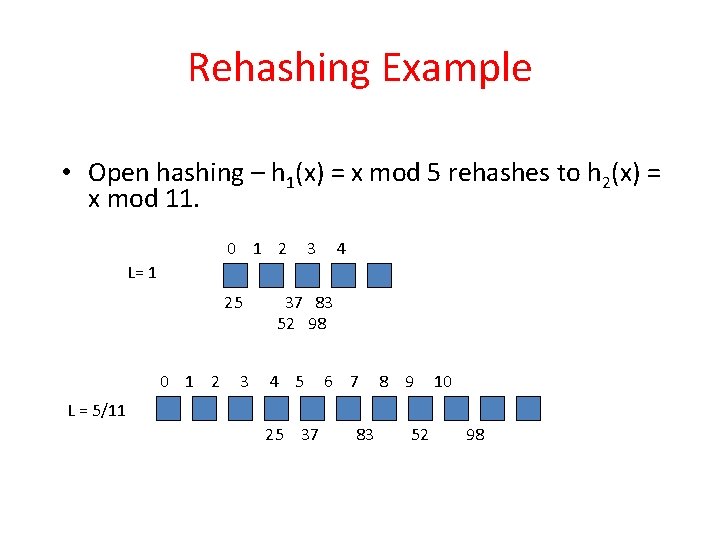
Rehashing Example • Open hashing – h 1(x) = x mod 5 rehashes to h 2(x) = x mod 11. 0 1 2 3 4 L= 1 25 0 1 2 3 37 83 52 98 4 5 6 7 8 9 10 L = 5/11 25 37 83 52 98

Rehashing Picture • Starting with table of size 2, double when load factor > 1 hashes rehashes 1 2 3 4 5 6 7 8 9 10 11 12 13 14 15 16 17 18 19 20 21 23 24 25 An expensive operation once in a while. .

Caveats • Hash functions are very often the cause of performance bugs. • Hash functions often make the code not portable. • If a particular hash function behaves badly on your data, then pick another.