MODELING AND FORECASTING STOCK RETURN VOLATILITY USING A

MODELING AND FORECASTING STOCK RETURN VOLATILITY USING A RANDOM LEVEL SHIFT MODEL Lu Hongda Yu Lu Meng Shuangshuang

Introduction Main goal : to forecast volatility proxied by daily squared returns Our approach: extends Starica and Granger (2005)’s work Apply log-absolute returns and daily returns rather than intra-daily data

Three main parts 1 2 3 • The model, the specification adopted and the estimation procedure • Estimation results and diagnostics • The forecasting comparisons

1. THE MODEL AND THE ESTIMATION METHOD Lu Hongda

1. 1 Model

1. 2 Assumptions

1. 3 Model Estimation

Then…

1. 3 Model Estimation

Continue…

And…

1. 4 The estimation method

1. 4 The estimation method where where 1 represents a (4*1 )vector of ones denotes element-by-element multiplication with element, with the element of

1. 4 The estimation method

1. 4 The estimation method Therefore, the evolution of is given by: Or more compactly by:

1. 4 The estimation method

1. 4 The estimation method The best forecast for the state variable and its associated variance conditional on past information and are We have the measurement equation

1. 4 The estimation method Where Hence, the prediction error and variance are: Applying standard updating formulae, we have (given ),

1. 4 The estimation method To reduce the dimension of the estimation problem, we adopt the re-collapsing procedure suggested by Harrison and Stevens (1976), given by

1. 4 The estimation method By doing so, we make unaffected by the history of states before time t − 1 If we define we then have four possible states corresponding to with the transition matrix Π as defined in (4)

1. 4 The estimation method The vector of conditional densities thus have a more compact representation given by: Where are as defined in (5)

1. 5. Apply model and estimation method

1. 5. Apply model and estimation method

1. 5. Apply model and estimation method

2. EMPIRICAL RESULTS FOR RETURNS ON STOCK MARKET INDICES Yu Lu

2. 1. Estimation results

Estimation results? Table 1: Maximum Likelihood Estimates S&P 500 0. 7524 0. 00198 0. 73995 (SD: ) 0. 74290 0. 00082 0. 73920 AMEX 0. 84579 0. 00157 0. 72346 (SD: ) 0. 85127 0. 00097 0. 70671 Dow Jones 0. 97270 0. 00120 0. 73291 (SD: ) 0. 94899 0. 00121 0. 73196 NASDAQ 1. 53121 0. 00081 0. 74280 (SD: ) 0. 00079 0. 74286 1. 53283 0. 00030 -0. 0146 -0. 00087 -0. 00029

2. 2. Noteworthy features of results:

2. 2. Noteworthy features of results:

2. 3. The effect of level shifts on longmemory and conditional heteroskedasticity Investigating whether the shifts can explain: a) the well-documented feature of long-memory b) the presence of conditional heteroskedasticity

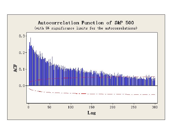
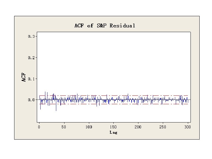
2. 3. 1. Effects of level shift on longmemory

The log-absolute returns clearly display an autocorrelation function that resembles that of a long-memory process: it decays very slowly and the values remain important even at lag 300.

For all practical purposes, we can view the short -memory component as being nearly white noise.

2. 3. 2 Effects of level shift on conditional heteroskedasticity

CGARCH model

Table 2. Parameter Estimates S&P 500 Coefficient Estimate Std. Error t-Statistic p-value No level shifts in GARCH 0. 057 0. 004 13. 55 0 0. 938 0. 004 214. 75 0 No level shifts in CGARCH 0. 058 0. 007 7. 98 0 0. 939 0. 009 95. 34 0 0. 9996 0. 0003 3250. 19 0 0. 027 0. 005 5. 36 0 -0. 085 0. 069 4. 73 0. 082 0. 525 0. 217 1. 54 0. 088 0. 622 0. 012 106. 98 0 0. 138 0. 089 2. 47 0. 031 Level shifts in CGARCH

2. 3. 2 Effects of level shift on conditional heteroskedasticity Use the standard GARCH (1, 1) model allow for level shifts(CGARCH)

Summary: The level shifts model with white noise errors appears to provide an accurate description of the data. The level shift component is an important feature that explains both the long-memory and conditional heteroskedasticity features generally perceived as stylized facts.

3 FORECASTING Performance of the level shift model &GARCH(1, 1)in forecasting volatility Meng Shuangshuang

3. 1 Design of forecasting experiment Following Starica and Granger(2005) Start forecasting at observations 2, 000 Re-estimate every 20 days, up to 200 days Proxy: realized squared returns( )

3. 2 Evaluation of forecasting performance evaluated by the ratio of their MSE: MSE(p) where n : no. of forecasting produced

3. 3 construction of the forecasts The level shift model(1) The level shift model an appropriate transformation where C : a positive constant used to bound returns away from zero yields

3. 3 construction of the forecasts The level shift model(2) continue ignore level shifts when forecasting rare uncertain about timing and magnitudes

3. 3 construction of the forecasts The level shift model(3) Continue the K -period ahead forecast of the squared returns is :

3. 3 construction of the forecasts The GARCH model(1) Student-t GARCH(1, 1) model Transformation:

3. 3 construction of the forecasts The GARCH model(2)

3. 4 Forecasting Comparisons The comparison indicates that with a precise estimate of the mean of log-absolute returns at a given date, we can obtain much better forecasts from the level shift model than the other models. random level shifts model the GARCH(1, 1) use the fitted means obtained from the full sample to get the mean re-estimate every 20 observations to get the mean

3. 4 Forecasting Comparisons Horizon P days S&P 500 20 0. 5 120 0. 51 40 0. 44 140 0. 54 60 0. 44 160 0. 56 80 0. 46 180 0. 59 100 0. 48 200 0. 62

3. 4 Forecasting Comparisons Table: volatility forecasting performance of the LS model & GARCH(1, 1) model ratio < 1 : volatility forecast of the LS model is more precise than the GARCH(1, 1) model The figure shows an over-all better longerhorizon volatility forecast performance of the LS model

Conclusion a simple estimation method for a model with a random level shift & a short-memory component The level shift component : explains the presence of both the long-memory and conditional heteroskedasticity a short-memory component: assume to be white noise impressive results : when model applied to logabsolute returns of many indices

Conclusion Volatility forecasting with the model: Ø improvement with squared returns as a proxy Ø Noticeable when mean is well estimated Ø Difficult to obtain precise estimates of the mean

END Thank you