Chap 9 Estimating Volatility Consolidated Approach Estimating Volatility

Chap 9 Estimating Volatility : Consolidated Approach

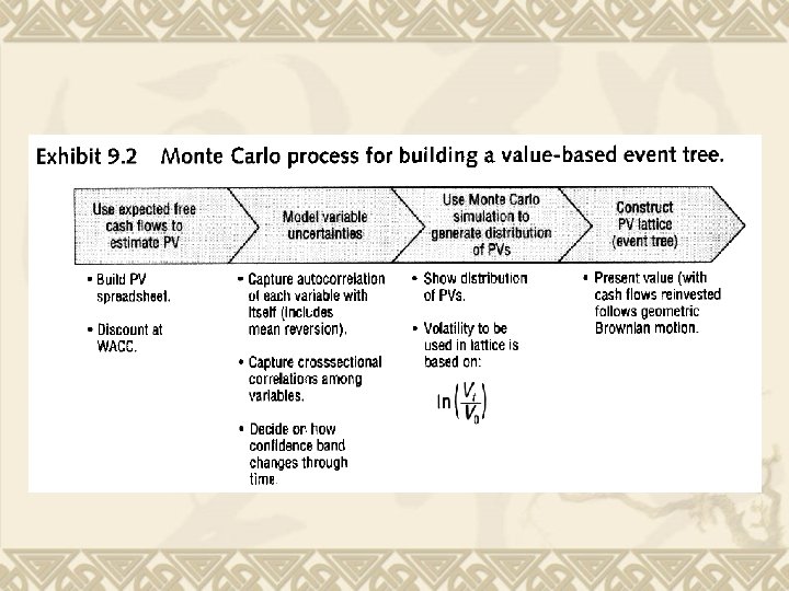
Estimating Volatility : Consolidated Approach v Volatility of a project is not the same as the volatility of any of the input variables, nor is it equal to the volatility of the company’s equity. v How to use a Monte Carlo approach to value a project. v Monte Carlo tools are fairly simple to use and can model the cross correlations among various inputs such as price and quantity, as well as time series properties such as mean reversion.

v Two approaches for estimating a consolidated measure of the volatility of a value-based event tree are discussed later in this chapter. v We call them the historical and the subjective approaches. v We use the term “consolidated” because the output is a single estimate of volatility, built up from the many uncertainties that contribute to it. v Estimates of these separate uncertainties are taken either from historical data, or from the subjective estimates of management.

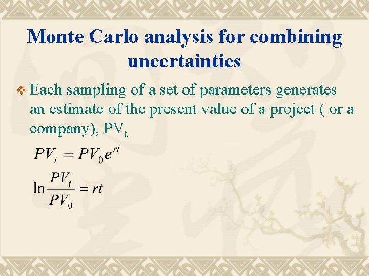
Monte Carlo analysis for combining uncertainties v Each sampling of a set of parameters generates an estimate of the present value of a project ( or a company), PVt

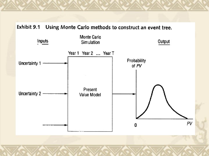
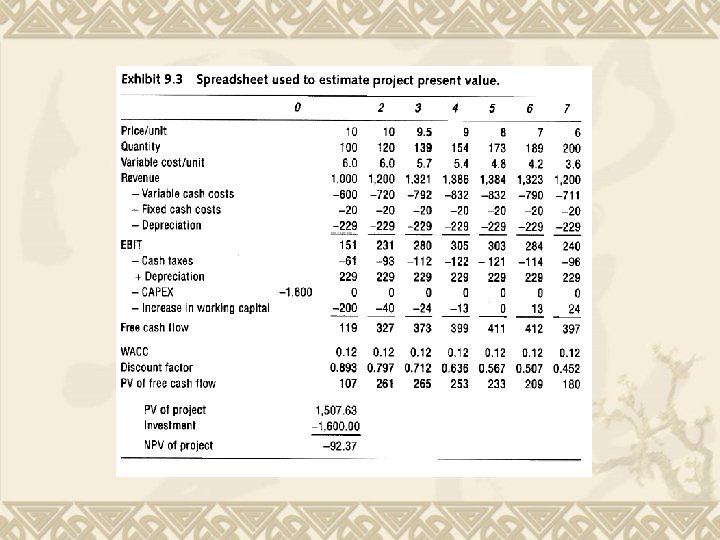
v We start with a present value spreadsheet, model the variable uncertainties, use the Monte Carlo simulation to estimate the standard deviation of rates of return, and then construct the event tree binomial lattice. v 1. Price per unit v 2. Quantity of output v 3. Variable cost per unit

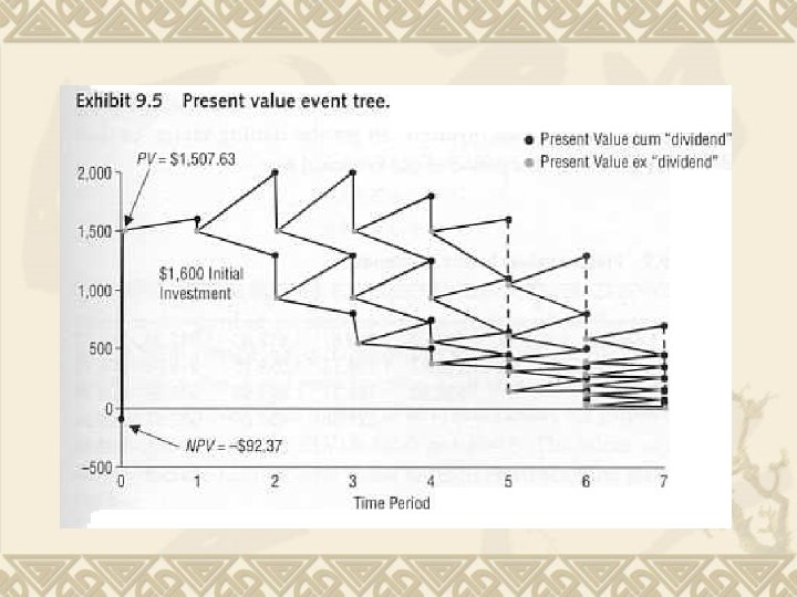
v If the weighted average cost of capital is 12 percent, the present value is $1, 507. 63; and if the investment outlay is $1, 600, the net present value is -$92. 37. v The expected price per unit starts out at $10, but declines over time due to anticipated competitive pressure. v The expected quantity sold grows at 20 percent in the year after the product is released, but despite price cuts, growth shows to 5. 8 percent in the last year of the forecast.

v The variable cost per unit is expected to decline from $6. 00 in the first year of operation to $3. 56 per unit in the last year. v They believe that their errors of estimation will be highly positively correlated through time (autocorrelation of 90%), implying that if they underestimate the price that is achievable in one year, they are highly likely to have underestimated it the next year as well.

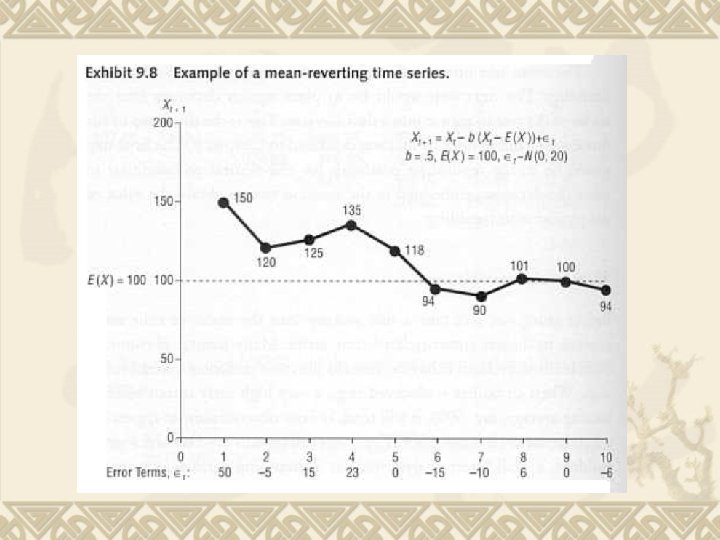
v This time dependence is called autocorrelation, and if it is negative, implying that a high value is more likely to be followed by a low value (and vice versa), then it is called mean reversion. v 1. Define Assumption. v 2. Set Autocorrelations. “correlate icon” Crystal Ball to “select an assumption” v 3. Define Forecast Variable.

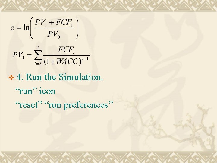
v 4. Run the Simulation. “run” icon “reset” “run preferences”

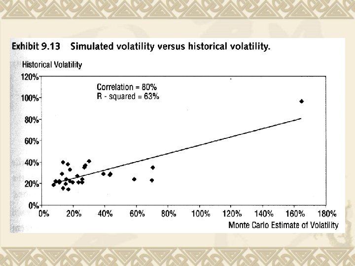
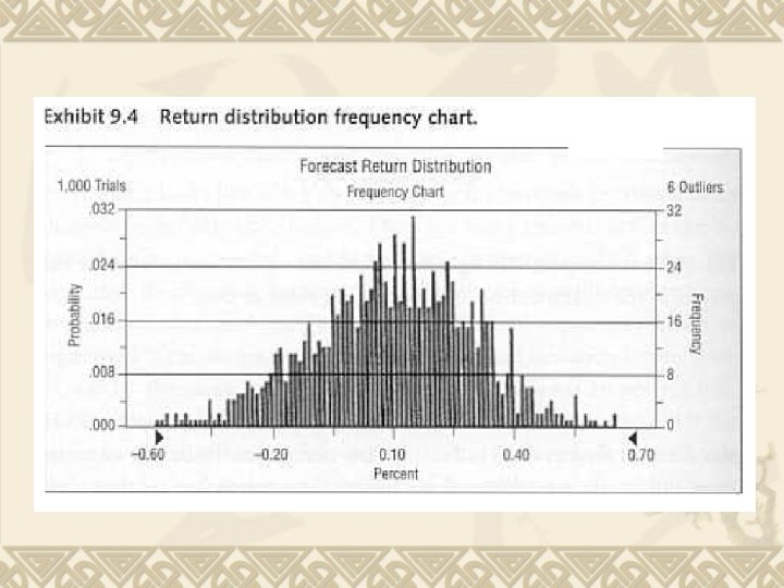
v The mean return was 13 percent, and the annual standard deviation was 21 percent. v The standard deviation of prices was equal to 10 percent, but the standard deviation of the rate of return on the project is 21 percent. v The input variables that drive uncertainty is not the same as the volatility of the project.

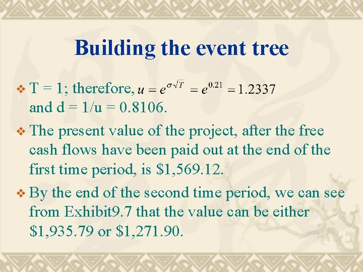
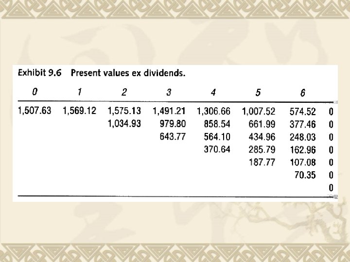
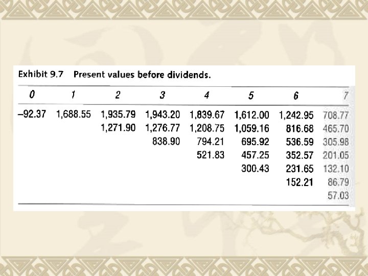
Building the event tree v. T = 1; therefore, and d = 1/u = 0. 8106. v The present value of the project, after the free cash flows have been paid out at the end of the first time period, is $1, 569. 12. v By the end of the second time period, we can see from Exhibit 9. 7 that the value can be either $1, 935. 79 or $1, 271. 90.

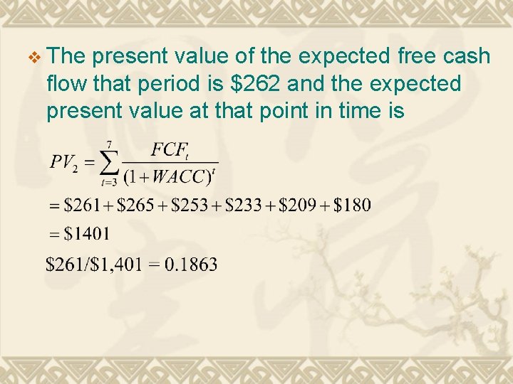
v The present value of the expected free cash flow that period is $262 and the expected present value at that point in time is

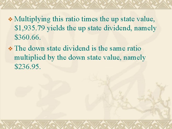
v Multiplying this ratio times the up state value, $1, 935. 79 yields the up state dividend, namely $360. 66. v The down state dividend is the same ratio multiplied by the down state value, namely $236. 95.

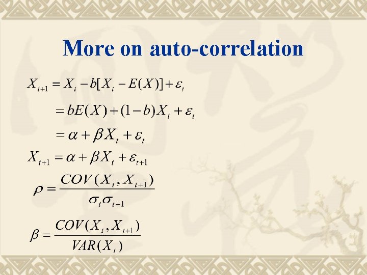
More on auto-correlation

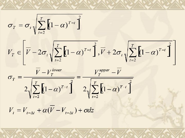
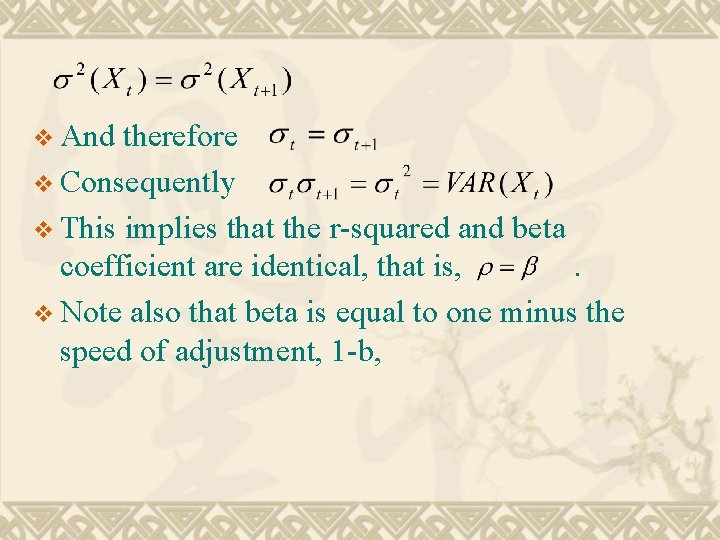
v And therefore v Consequently v This implies that the r-squared and beta coefficient are identical, that is, . v Note also that beta is equal to one minus the speed of adjustment, 1 -b,

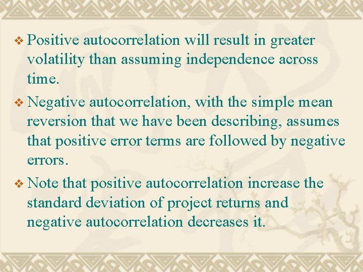
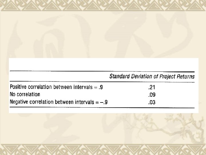
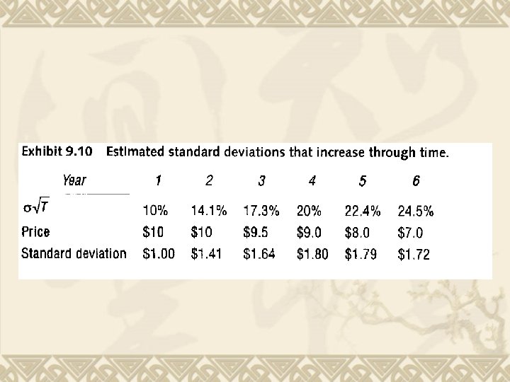
v Positive autocorrelation will result in greater volatility than assuming independence across time. v Negative autocorrelation, with the simple mean reversion that we have been describing, assumes that positive error terms are followed by negative errors. v Note that positive autocorrelation increase the standard deviation of project returns and negative autocorrelation decreases it.

Using historical data v Use the r-squared of the time serious regression to capture the autocorrelation effect. v Cross-correlation between variables is captured by the r-squared between them. v The standard deviation for each of the variables is the standard deviation of the residuals that results from the time serious regression.

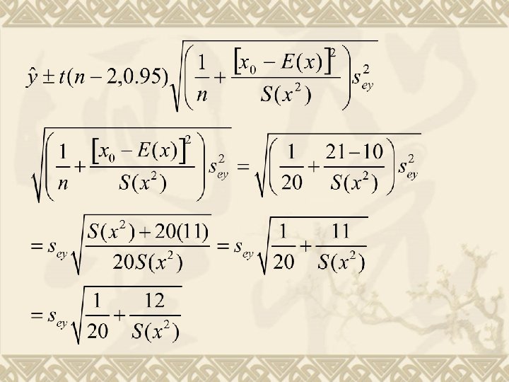
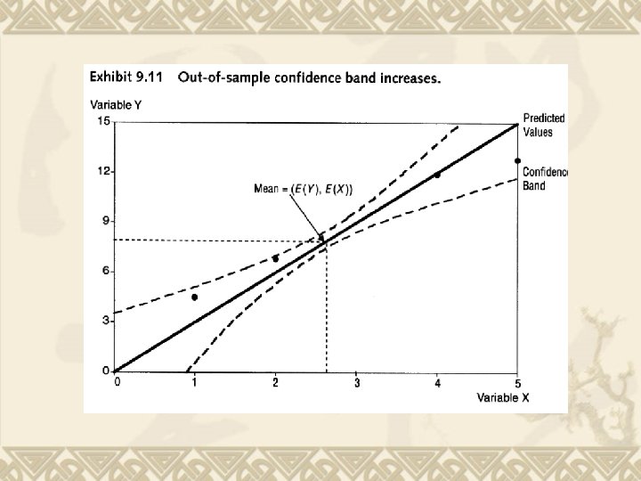
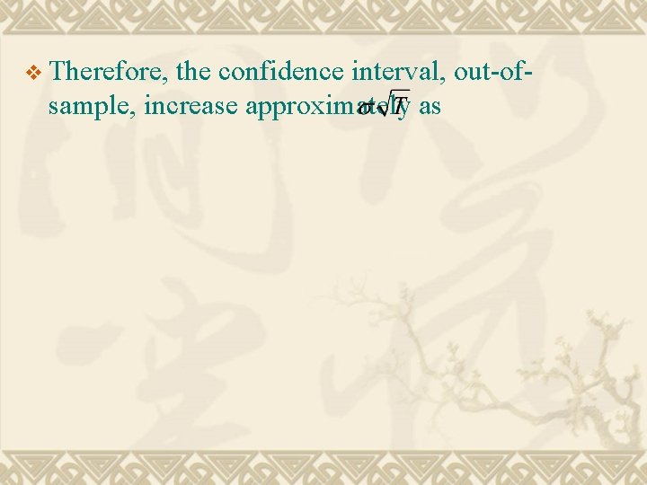
v Therefore, the confidence interval, out-ofsample, increase approximately as

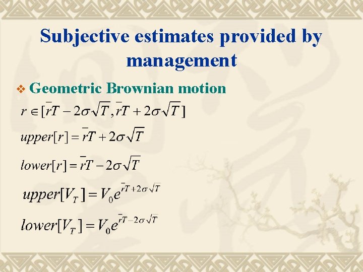
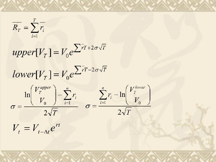
Subjective estimates provided by management v Geometric Brownian motion

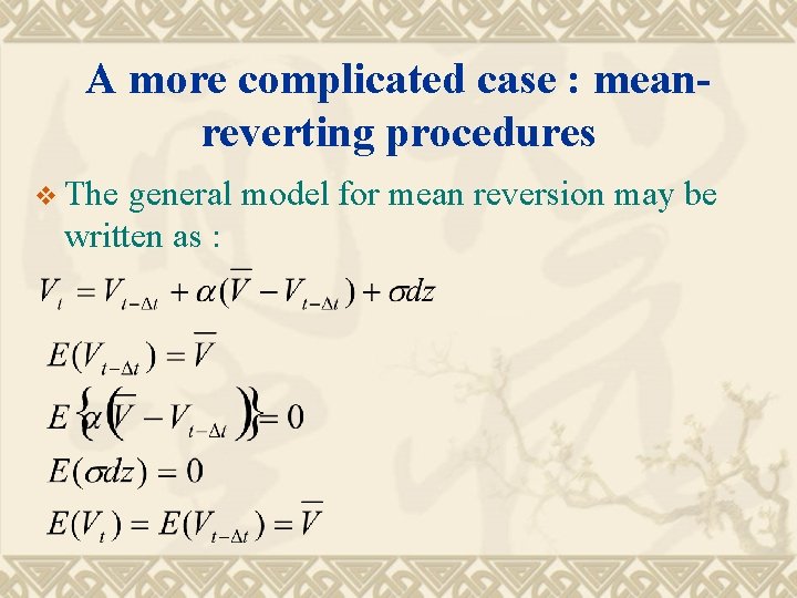
A more complicated case : meanreverting procedures v The general model for mean reversion may be written as :