MCFM and techniques for oneloop diagrams R Keith

MCFM and techniques for one-loop diagrams. R. Keith Ellis Fermilab Berkeley Workshop on Boson+Jets Production, March 2008

http: //mcfm. fnal. gov/ MCFM overview Monte Carlo for Fe. Mtobarn processes. At LHC few of the cross sections are expressed in fb, so MCFM. Parton level cross sections predicted to NLO in S. Currently released version 5. 2, July 2007 Features-Less sensitivity to unphysical R and F, better normalization for rates, fully differential distributions. Shortcomings- low parton multiplicity (no showering), no hadronization, hard to model detector effects. Work by John Campbell and Keith Ellis with appearances by guest celebrities, Fabio Maltoni, Francesco Tramontano, Scott Willenbrock & Giulia Zanderighi.

' W, Z + jet processes available in MCFM + specific processes involving heavy quark distributions in the initial state (cf Maltoni)

Why NLO? • Less sensitivity to unphysical input scales (eg. renormalization and factorization scales). • First real prediction of normalization of observables occurs at NLO. • It is a necessary prerequisite for other techniques, matching with resummed calculations, (MC@NLO, POWHEG, etc). • More physics (a) parton merging to give structure in jets, (b) initial state radiation, (c) More species of incoming partons enter at NLO.

Improved scale dependence • • Variations of renormalization scale are themselves NLO effects. So without NLO calculation one has no idea about the choice of renormalization (or factorization) scale. Example: Top cross section at the Tevatron. Performing the calculation at NLO reduces the dependence on unphysical scales. is the renormalization and factorization scale.

W+n jet rates from CDF Both uncertainty on rates and deviation of Data/Theory from 1 are smaller than other calculations. “Berends” ratio agrees well for all calculations, but unfortunately only available for n 2 from MCFM.

PRD 77 011108 R CDF results for W+jets Ratio of data over theory (MCFM) for first and second jet appears to agree well. MCFM results are not available at NLO for third jet.

Z + n jets rate agrees well with NLO QCD from MCFM

Recent additions to MCFM • WW+1 jet (Campbell, RKE, Zanderighi, ar. Xiv: 0710. 1832) • H+2 jet (Campbell, RKE, Zanderighi, hep-ph/0608194) Unfortunately neither of these processes are yet included in the publically released code.

Campbell et al, ar. Xiv: 0710. 1832 [hep-ph] Dittamaier et al, ar. Xiv: 0710. 1577 [hep-ph] WW+1 jet WW+1 jet and impact on Higgs ->WW + 1 jet search Rates with cuts I+II Standard Cuts I : Cuts II:

Campbell, Ellis, Zanderighi Higgs+2 jets at NLO • Calculation performed using an effective Lagrangian, valid in the large mt limit. Three basic processes at lowest order.

Higgs + 2 jet continued • NLO corrections are quite mild, increasing LO cross section by 15% • NLO cross section contains a considerable residual scale uncertainty.

Higgs + 2 jets rapidity distribution versus WBF • Shape of NLO result, similar to LO in rapidity. • WBF shape is quite different at NLO.

Extension to higher leg processes • MCFM does not include W/Z+3 jets, W/Z+4 jets at NLO. • We know the tree graphs, we know the subtraction procedure, with enough effort we can write an efficient phase space generator. • The bottleneck is the calculation of multi-leg, one-loop diagrams. • Straightforward numerical integration of one-loop diagrams is complicated, by the presence of soft, collinear and UV divergences • Analytic calculation may be too painstaking. • Our preferred method is a semi-numerical approach. Scalar integrals are calculated analytically and their coefficients calculated numerically.

The calculation of one loop amplitudes • The classical paradigm for the calculation of one-loop diagrams was established in 1979. • Complete calculation of one-loop scalar integrals • Reduction of tensors oneloop integrals to scalars. Neither will be adequate for present-day purposes.

Techniques for one loop diagrams • QCDLoop project: allows one to calculate an arbitrary one-loop scalar integral (work with Giulia Zanderighi) • Unitarity techniques for one-loop amplitudes Ossola, Papadopoulos, Pittau & work with Giele, Kunszt, Melnikov

Scalar one-loop integrals • ‘t Hooft and Veltman’s integrals contain internal masses; however in QCD many lines are (approximately) massless. The consequent soft and collinear divergences are regulated by dimensional regularization. • So we need general expressions for boxes, triangles, bubbles and tadpoles, including the cases with one or more vanishing internal masses.

Scalar triangle integrals Y is the modified Cayley matrix

Basis set of divergent integrals By classsifying the integral in terms of the number of zero internal masses, and the number of distinct Cayley matrices we can create a basis set of divergent integrals The basis set of divergent triangles contains 6 integrals

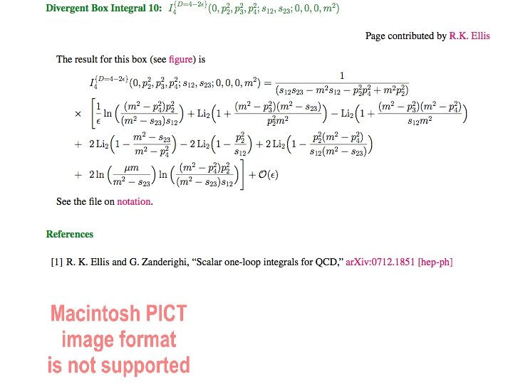
Similarly, the modified Cayley matrices for 16 divergent box integrals

The basis set of box integrals contains 16 integrals.

QCDLoop. fnal. gov QCDLoop web page giving access to hyper-linked PDF web-pages which give the results for the basis integrals, together with references, special cases etc. 11 of the 16 divergent box integrals were known in the literature. The rest are new.

Fortran code is available. It calculates finite integrals using the ff library, and calculates divergent integrals using the QCDLoop library.

Numerical checks We can perform a numerical check of the code, by using the Relation between boxes, triangles and the six-dimensional box. In D=6, the box integral is finite - no UV, IR or collinear divergences So we can check this relation numerically, (including in the physical Region by setting the causal equal to a very small number.

Basis set of scalar integrals Any one-loop amplitude can be written as a linear sum of boxes, triangles, bubbles and tadpoles In addition, in the context of NLO calculations, scalar higher point functions, can always be expressed as sums of box integrals. Passarino, Veltman - Melrose (‘ 65) • Scalar hexagon can be written as a sum of six pentagons. • For the purposes of NLO calculations, the scalar pentagon can be written as a sum of five boxes. • In addition to the ‘t. H-V integrals we need integrals containing infrared and collinear divergences.

Algebraic reduction, subtraction terms • Ossola, Papadopoulos and Pittau showed that there is a systematic way of calculating the subtraction terms at the integrand level. • We can re-express the rational function in an expansion over 4, 3, 2, and 1 propagator terms. • The residues of these pole terms contain the l-independent master integral coefficients plus a finite number of spurious terms.

Decomposing in terms of … • Without the integral sign, the identification of the coefficients is straightforward. • Determine the coefficients of a multipole rational function.

Reduction at the integrand level Spurious terms: residual l-dependence Finite number of spurious terms: 1 (box), 6 (triangle) 8 (bubble) 2 unknowns 7 unknowns Products of tree amplitudes Suitable for numerical evaluation for cut-constructible part

Residues of poles and unitarity cuts Define residue function We can determine the d-coefficients, then the c-coefficients and so on

van Neerven-Vermaseren basis Example: solve for the box coefficients by setting We find two complex solutions The most general form of the residue is

Ellis, Giele, Kunszt Result for six gluon amplitude • Results shown here for the cutconstructible part • The relative error for the finite part of the 6 -gluon amplitude compared to the analytic result, for the (+ + - -) helicity choice. The horizontal axis is the log of the relative error, the vertical axis is the number of events in arbitrary linear units. • For most events the error is less than 10 -6, although there is a tail extending to higher error.

Giele, Kunszt, Melnikov, ar. Xiv 0801. 2237 Extension to full amplitude • Keep dimensions of virtual unobserved particles integer and perform calculations in more than one dimension. • Arrive at non-integer values D=4 -2 by polynomial interpolation. • Results for six-gluon amplitudes agree with original Feynman diagram calculation of RKE, Giele, Zanderighi.

Summary • MCFM appears to describe untagged W/Z+1 jet and W/Z+2 jet data well. • Even at the Tevatron the known results on multi-leg processes are inadequate. • Calculation of one-loop scalar integrals is complete. • There is much theoretical effort on the calculation of oneloop multi-leg diagrams. • Practical calculations have used either a) analytic results, b) PV reduction, or c) Giele-Glover style reduction. • However semi-numerical unitarity-based methods show great promise for the future.