Management Science MNG 221 Linear Programming The Simplex

Management Science – MNG 221 Linear Programming – The Simplex Method

The Simplex Method • The Simplex Method, is a general mathematical solution technique for solving linear programming problems. • The model is put into the form of a table, and then a number of mathematical steps are performed on the table. • It replicates the process in graphical analysis of moving from one extreme point on the solution boundary to another.

The Simplex Method • Unlike the graphical method, in which we could simply search through all the solution points to find the best one, the simplex method moves from one better solution to another until the best one is found, and then it stops. • The first step in solving a linear programming model manually with the simplex method is to convert the model into standard form

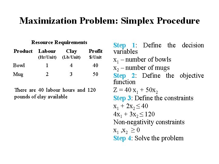
Maximization Problem: Simplex Procedure Resource Requirements Product Labour Clay Profit (Hr/Unit) (Lb/Unit) $/Unit Bowl 1 4 40 Mug 2 3 50 There are 40 labour hours and 120 pounds of clay available Step 1: Define the decision variables x 1 – number of bowls x 2 – number of mugs Step 2: Define the objective function Z = 40 x 1 + 50 x 2 Step 3: Define the constraints x 1 + 2 x 2 ≤ 40 4 x 1 + 3 x 2 ≤ 120 Non-negativity constraints x 1 , x 2 ≥ 0 Step 4: Solve the problem

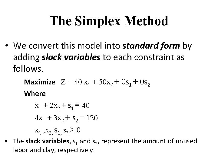
The Simplex Method • We convert this model into standard form by adding slack variables to each constraint as follows. Maximize Z = 40 x 1 + 50 x 2 + 0 s 1 + 0 s 2 Where x 1 + 2 x 2 + s 1 = 40 4 x 1 + 3 x 2 + s 2 = 120 x 1 , x 2, s 1, s 2 ≥ 0 • The slack variables, s 1 and s 2, represent the amount of unused labor and clay, respectively.

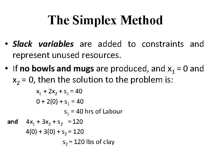
The Simplex Method • Slack variables are added to constraints and represent unused resources. • If no bowls and mugs are produced, and x 1 = 0 and x 2 = 0, then the solution to the problem is: x 1 + 2 x 2 + s 1 = 40 0 + 2(0) + s 1 = 40 hrs of Labour and 4 x 1 + 3 x 2 + s 2 = 120 4(0) + 3(0) + s 2 = 120 lbs of clay

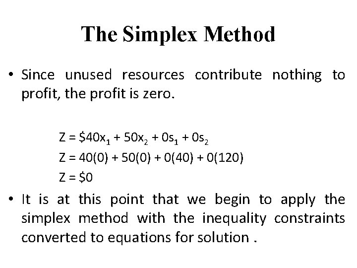
The Simplex Method • Since unused resources contribute nothing to profit, the profit is zero. Z = $40 x 1 + 50 x 2 + 0 s 1 + 0 s 2 Z = 40(0) + 50(0) + 0(40) + 0(120) Z = $0 • It is at this point that we begin to apply the simplex method with the inequality constraints converted to equations for solution.

The Simplex Method – The Solution of Simultaneous Equations • The equations should be solved simultaneously to determine the values of the variables at every possible solution point. • Our Example problem has two equations and four unknowns (i. e. , two decision variables and two slack variables) • This situation makes direct simultaneous solution impossible.

The Simplex Method – The Solution of Simultaneous Equations • The simplex method alleviates this problem by assigning some of the variables a value of zero. • The number of variables assigned values of zero is n - m, where: n = the number of variables m = the number of constraints (excluding the non-negativity constraints). n = 4 variables & m = 2 constraints; • Therefore, two of the variables are assigned a value of zero (i. e. , 4 - 2 = 2).

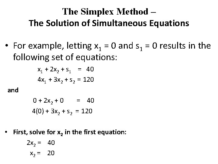
The Simplex Method – The Solution of Simultaneous Equations • For example, letting x 1 = 0 and s 1 = 0 results in the following set of equations: x 1 + 2 x 2 + s 1 = 40 4 x 1 + 3 x 2 + s 2 = 120 and 0 + 2 x 2 + 0 = 40 4(0) + 3 x 2 + s 2 = 120 • First, solve for x 2 in the first equation: 2 x 2 = 40 x 2 = 20

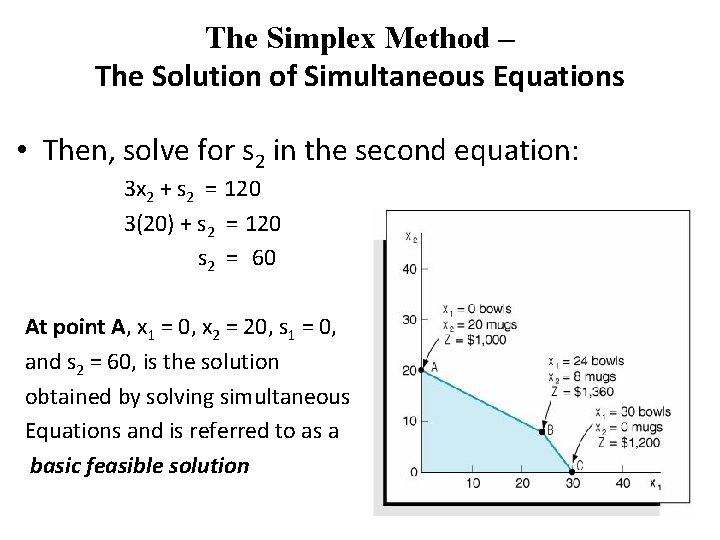
The Simplex Method – The Solution of Simultaneous Equations • Then, solve for s 2 in the second equation: 3 x 2 + s 2 = 120 3(20) + s 2 = 120 s 2 = 60 At point A, x 1 = 0, x 2 = 20, s 1 = 0, and s 2 = 60, is the solution obtained by solving simultaneous Equations and is referred to as a basic feasible solution

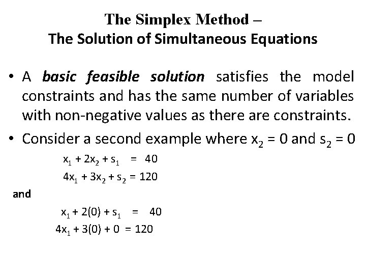
The Simplex Method – The Solution of Simultaneous Equations • A basic feasible solution satisfies the model constraints and has the same number of variables with non-negative values as there are constraints. • Consider a second example where x 2 = 0 and s 2 = 0 x 1 + 2 x 2 + s 1 = 40 4 x 1 + 3 x 2 + s 2 = 120 and x 1 + 2(0) + s 1 = 40 4 x 1 + 3(0) + 0 = 120

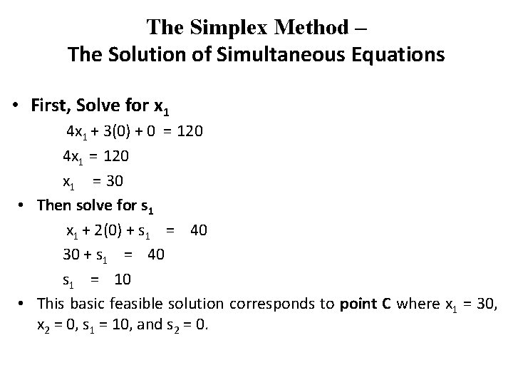
The Simplex Method – The Solution of Simultaneous Equations • First, Solve for x 1 4 x 1 + 3(0) + 0 = 120 4 x 1 = 120 x 1 = 30 • Then solve for s 1 x 1 + 2(0) + s 1 = 40 30 + s 1 = 40 s 1 = 10 • This basic feasible solution corresponds to point C where x 1 = 30, x 2 = 0, s 1 = 10, and s 2 = 0.

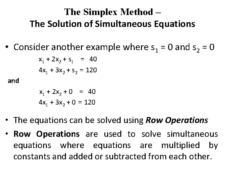
The Simplex Method – The Solution of Simultaneous Equations • Consider another example where s 1 = 0 and s 2 = 0 x 1 + 2 x 2 + s 1 = 40 4 x 1 + 3 x 2 + s 2 = 120 and x 1 + 2 x 2 + 0 = 40 4 x 1 + 3 x 2 + 0 = 120 • The equations can be solved using Row Operations • Row Operations are used to solve simultaneous equations where equations are multiplied by constants and added or subtracted from each other.

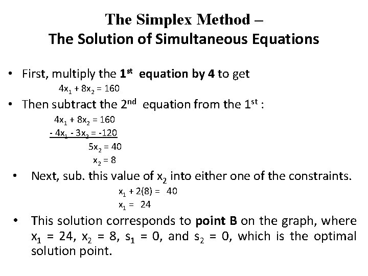
The Simplex Method – The Solution of Simultaneous Equations • First, multiply the 1 st equation by 4 to get 4 x 1 + 8 x 2 = 160 • Then subtract the 2 nd equation from the 1 st : 4 x 1 + 8 x 2 = 160 - 4 x 1 - 3 x 2 = -120 5 x 2 = 40 x 2 = 8 • Next, sub. this value of x 2 into either one of the constraints. x 1 + 2(8) = 40 x 1 = 24 • This solution corresponds to point B on the graph, where x 1 = 24, x 2 = 8, s 1 = 0, and s 2 = 0, which is the optimal solution point.

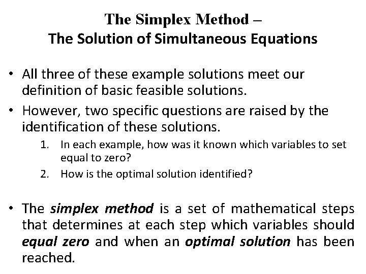
The Simplex Method – The Solution of Simultaneous Equations • All three of these example solutions meet our definition of basic feasible solutions. • However, two specific questions are raised by the identification of these solutions. 1. In each example, how was it known which variables to set equal to zero? 2. How is the optimal solution identified? • The simplex method is a set of mathematical steps that determines at each step which variables should equal zero and when an optimal solution has been reached.

LINEAR PROGRAMMING THE SIMPLEX METHOD

The Simplex Method • The steps of the simplex method are carried out within the framework of a table, or tableau. • The tableau organizes the model into a form that makes applying the mathematical steps easier. • The simplex method is a set of mathematical steps for solving a linear programming problem carried out in a table called a simplex tableau.

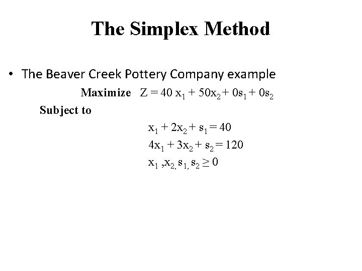
The Simplex Method • The Beaver Creek Pottery Company example Maximize Z = 40 x 1 + 50 x 2 + 0 s 1 + 0 s 2 Subject to x 1 + 2 x 2 + s 1 = 40 4 x 1 + 3 x 2 + s 2 = 120 x 1 , x 2, s 1, s 2 ≥ 0

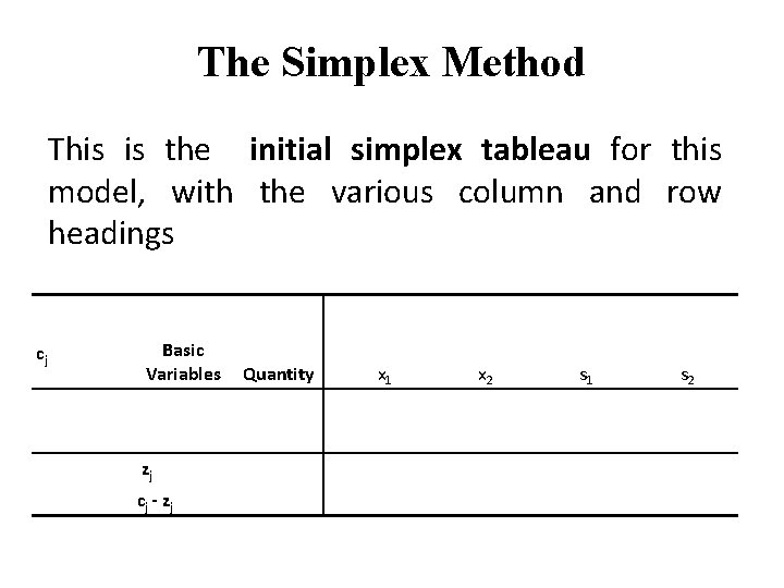
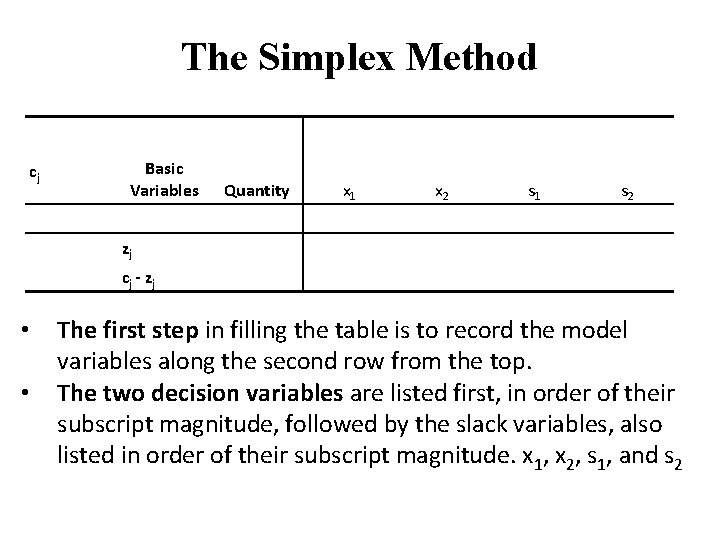
The Simplex Method This is the initial simplex tableau for this model, with the various column and row headings cj Basic Variables x 1 Quantity x 2 s 1 s 2 zj cj - zj

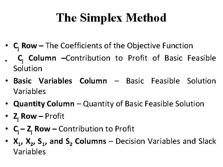
The Simplex Method • Cj Row – The Coefficients of the Objective Function • Cj Column –Contribution to Profit of Basic Feasible Solution • Basic Variables Column – Basic Feasible Solution Variables • Quantity Column – Quantity of Basic Feasible Solution • Zj Row – Profit • Cj – Zj Row – Contribution to Profit • X 1, X 2, S 1, and S 2 Columns – Decision Variables and Slack Variables

The Simplex Method cj Basic Variables x 1 Quantity x 2 s 1 s 2 zj cj - zj • • The first step in filling the table is to record the model variables along the second row from the top. The two decision variables are listed first, in order of their subscript magnitude, followed by the slack variables, also listed in order of their subscript magnitude. x 1, x 2, s 1, and s 2

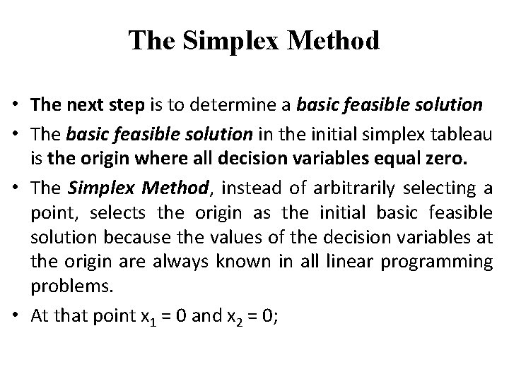
The Simplex Method • The next step is to determine a basic feasible solution • The basic feasible solution in the initial simplex tableau is the origin where all decision variables equal zero. • The Simplex Method, instead of arbitrarily selecting a point, selects the origin as the initial basic feasible solution because the values of the decision variables at the origin are always known in all linear programming problems. • At that point x 1 = 0 and x 2 = 0;

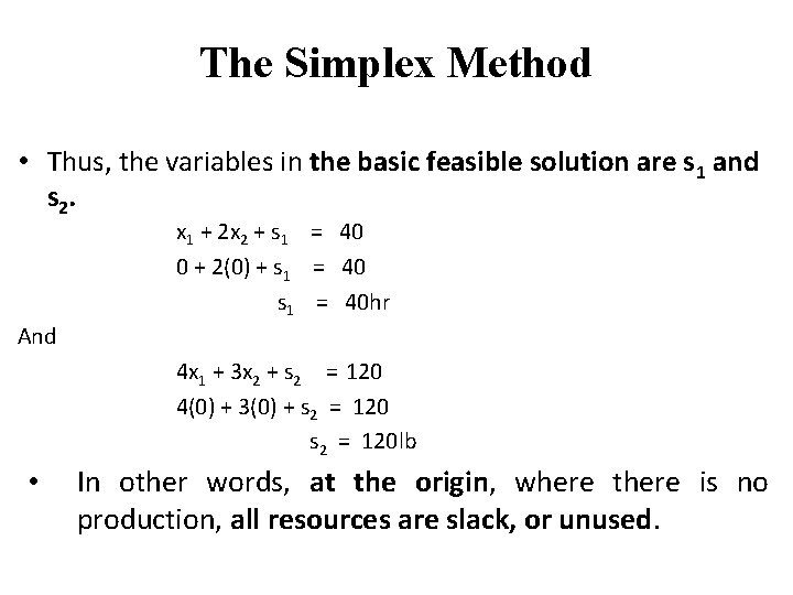
The Simplex Method • Thus, the variables in the basic feasible solution are s 1 and s 2. x 1 + 2 x 2 + s 1 = 40 0 + 2(0) + s 1 = 40 hr And 4 x 1 + 3 x 2 + s 2 = 120 4(0) + 3(0) + s 2 = 120 lb • In other words, at the origin, where there is no production, all resources are slack, or unused.

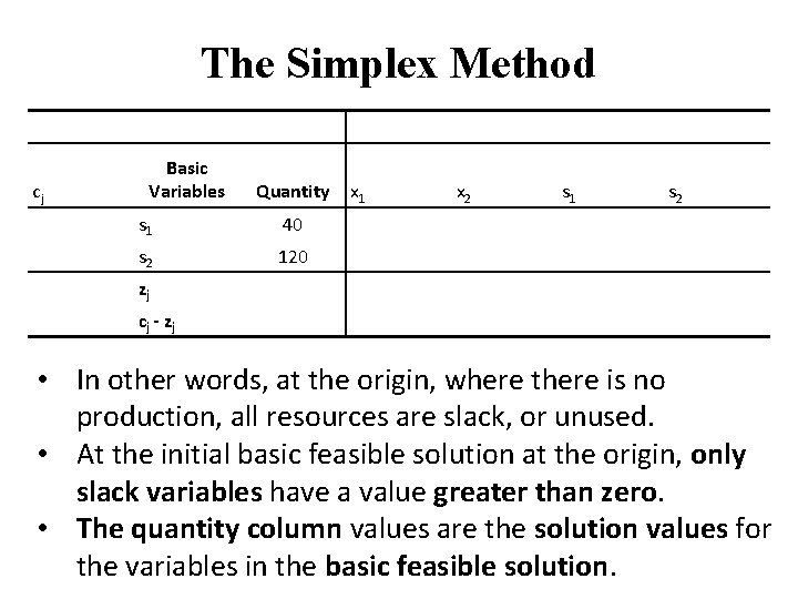
The Simplex Method cj Basic Variables Quantity x 1 s 1 40 s 2 120 zj cj - zj x 2 s 1 s 2 • In other words, at the origin, where there is no production, all resources are slack, or unused. • At the initial basic feasible solution at the origin, only slack variables have a value greater than zero. • The quantity column values are the solution values for the variables in the basic feasible solution.

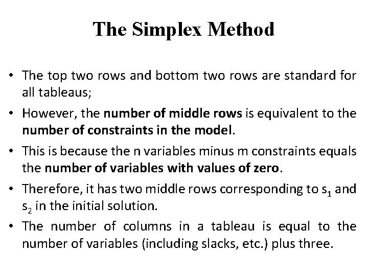
The Simplex Method • The top two rows and bottom two rows are standard for all tableaus; • However, the number of middle rows is equivalent to the number of constraints in the model. • This is because the n variables minus m constraints equals the number of variables with values of zero. • Therefore, it has two middle rows corresponding to s 1 and s 2 in the initial solution. • The number of columns in a tableau is equal to the number of variables (including slacks, etc. ) plus three.

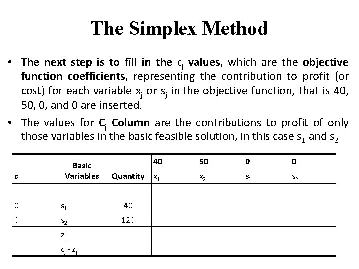
The Simplex Method • The next step is to fill in the cj values, which are the objective function coefficients, representing the contribution to profit (or cost) for each variable xj or sj in the objective function, that is 40, 50, 0, and 0 are inserted. • The values for Cj Column are the contributions to profit of only those variables in the basic feasible solution, in this case s 1 and s 2 cj Basic Variables 40 50 0 0 Quantity x 1 x 2 s 1 s 2 0 s 1 40 0 s 2 120 zj cj - zj

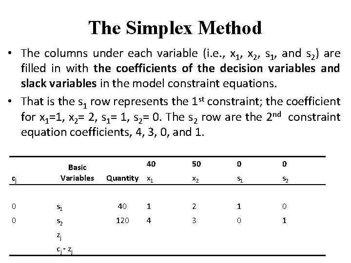
The Simplex Method • The columns under each variable (i. e. , x 1, x 2, s 1, and s 2) are filled in with the coefficients of the decision variables and slack variables in the model constraint equations. • That is the s 1 row represents the 1 st constraint; the coefficient for x 1=1, x 2= 2, s 1= 1, s 2= 0. The s 2 row are the 2 nd constraint equation coefficients, 4, 3, 0, and 1. cj Basic Variables 40 50 0 0 Quantity x 1 x 2 s 1 s 2 0 s 1 40 1 2 1 0 0 s 2 120 4 3 0 1 zj cj - zj

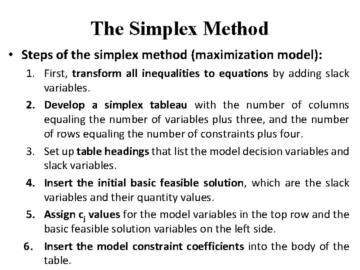
The Simplex Method • Steps of the simplex method (maximization model): 1. First, transform all inequalities to equations by adding slack variables. 2. Develop a simplex tableau with the number of columns equaling the number of variables plus three, and the number of rows equaling the number of constraints plus four. 3. Set up table headings that list the model decision variables and slack variables. 4. Insert the initial basic feasible solution, which are the slack variables and their quantity values. 5. Assign cj values for the model variables in the top row and the basic feasible solution variables on the left side. 6. Insert the model constraint coefficients into the body of the table.

LINEAR PROGRAMMING THE SIMPLEX METHOD Computing the zj and cj - zj Rows

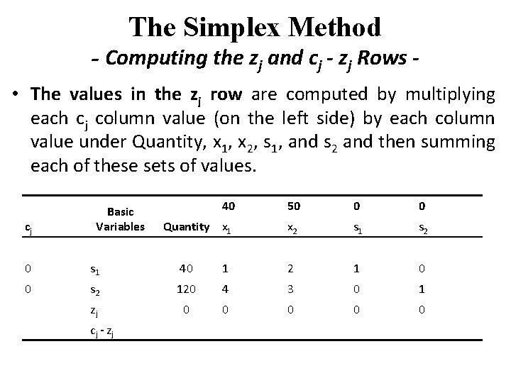
The Simplex Method - Computing the zj and cj - zj Rows • The values in the zj row are computed by multiplying each cj column value (on the left side) by each column value under Quantity, x 1, x 2, s 1, and s 2 and then summing each of these sets of values. cj Basic Variables 40 50 0 0 Quantity x 1 x 2 s 1 s 2 0 s 1 40 1 2 1 0 0 s 2 120 4 3 0 1 zj 0 0 0 cj - zj

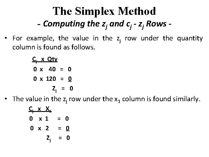
The Simplex Method - Computing the zj and cj - zj Rows • For example, the value in the zj row under the quantity column is found as follows. Cj x Qty 0 x 40 = 0 0 x 120 = 0 Zj = 0 • The value in the zj row under the x 1 column is found similarly. Cj x X 1 0 x 1 = 0 x 2 = 0 Zj = 0

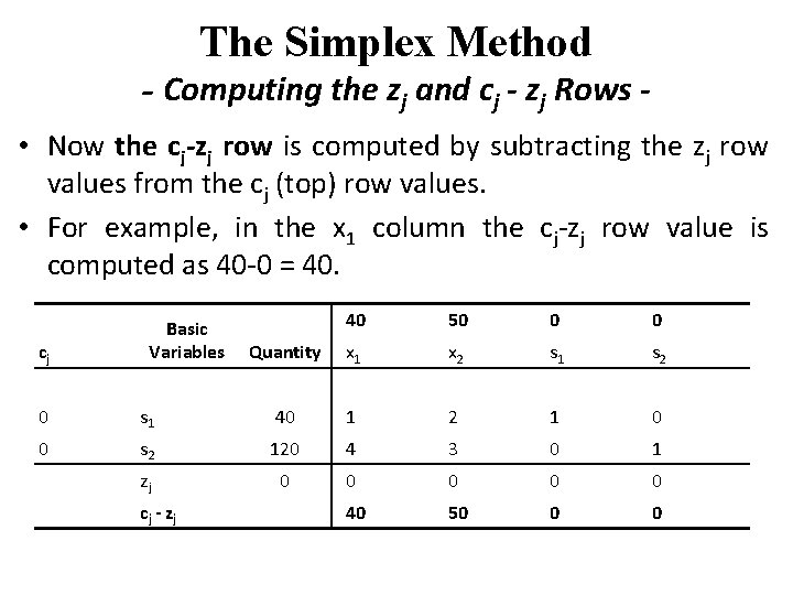
The Simplex Method - Computing the zj and cj - zj Rows • Now the cj-zj row is computed by subtracting the zj row values from the cj (top) row values. • For example, in the x 1 column the cj-zj row value is computed as 40 -0 = 40. cj Basic Variables 40 50 0 0 Quantity x 1 x 2 s 1 s 2 0 s 1 40 1 2 1 0 0 s 2 120 4 3 0 1 zj 0 0 0 cj - zj 40 50 0 0

The Simplex Method - Computing the zj and cj - zj Rows • This tableau represents the solution at the origin, where x 1 = 0, x 2 = 0, s 1 = 40, and s 2 = 120. • This solution is obviously not optimal because no profit is being made. • Thus, we want to move to a solution point that will give a better solution. • In other words, we want to produce either some bowls (x 1) or some mugs (x 2). • One of the nonbasic variables (i. e. , variables not in the present basic feasible solution) will enter the solution and become basic.

LINEAR PROGRAMMING THE SIMPLEX METHOD The Entering Non-basic Variable

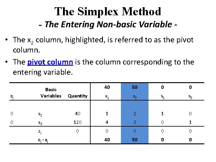
The Simplex Method - The Entering Non-basic Variable • The variable with the largest positive cj-zj value is The Entering Variable. • The cj-zj row values represent the net increase per unit of entering a nonbasic variable into the basic solution. • Because the objective is to maximize profit we enter the variable that will give the greatest net increase in profit per unit. • We select variable x 2 as the entering basic variable because it has the greatest net increase in profit per unit, $50 the highest positive value in the cj-zj row.

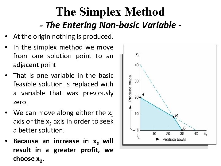
The Simplex Method - The Entering Non-basic Variable • At the origin nothing is produced. • In the simplex method we move from one solution point to an adjacent point • That is one variable in the basic feasible solution is replaced with a variable that was previously zero. • We can move along either the x 1 axis or the x 2 axis in order to seek a better solution. • Because an increase in x 2 will result in a greater profit, we choose x 2.

The Simplex Method - The Entering Non-basic Variable • The x 2 column, highlighted, is referred to as the pivot column. • The pivot column is the column corresponding to the entering variable. cj Basic Variables 40 50 0 0 Quantity x 1 x 2 s 1 s 2 0 s 1 40 1 2 1 0 0 s 2 120 4 3 0 1 zj 0 0 0 cj - zj 40 50 0 0

LINEAR PROGRAMMING THE SIMPLEX METHOD The Leaving Basic Variable

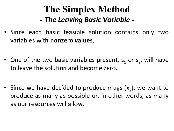
The Simplex Method - The Leaving Basic Variable • Since each basic feasible solution contains only two variables with nonzero values, • One of the two basic variables present, s 1 or s 2, will have to leave the solution and become zero. • Since we have decided to produce mugs (x 2), we want to produce as many as possible or, in other words, as many as our resources will allow.

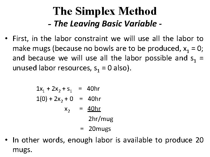
The Simplex Method - The Leaving Basic Variable • First, in the labor constraint we will use all the labor to make mugs (because no bowls are to be produced, x 1 = 0; and because we will use all the labor possible and s 1 = unused labor resources, s 1 = 0 also). 1 x 1 + 2 x 2 + s 1 = 40 hr 1(0) + 2 x 2 + 0 = 40 hr x 2 = 40 hr 2 hr/mug = 20 mugs • In other words, enough labor is available to produce 20 mugs.

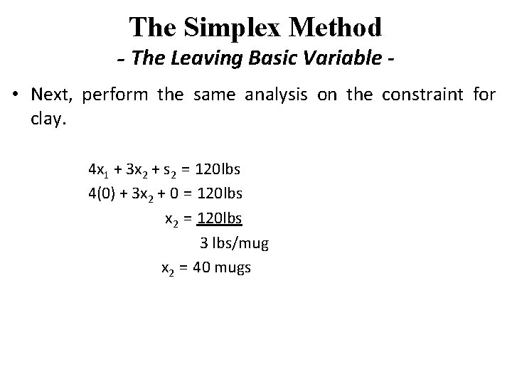
The Simplex Method - The Leaving Basic Variable • Next, perform the same analysis on the constraint for clay. 4 x 1 + 3 x 2 + s 2 = 120 lbs 4(0) + 3 x 2 + 0 = 120 lbs x 2 = 120 lbs 3 lbs/mug x 2 = 40 mugs

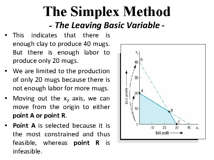
The Simplex Method - The Leaving Basic Variable - • This indicates that there is enough clay to produce 40 mugs. But there is enough labor to produce only 20 mugs. • We are limited to the production of only 20 mugs because there is not enough labor for more mugs. • Moving out the x 2 axis, we can move from the origin to either point A or point R. • Point A is selected because it is the most constrained and thus feasible, whereas point R is infeasible.

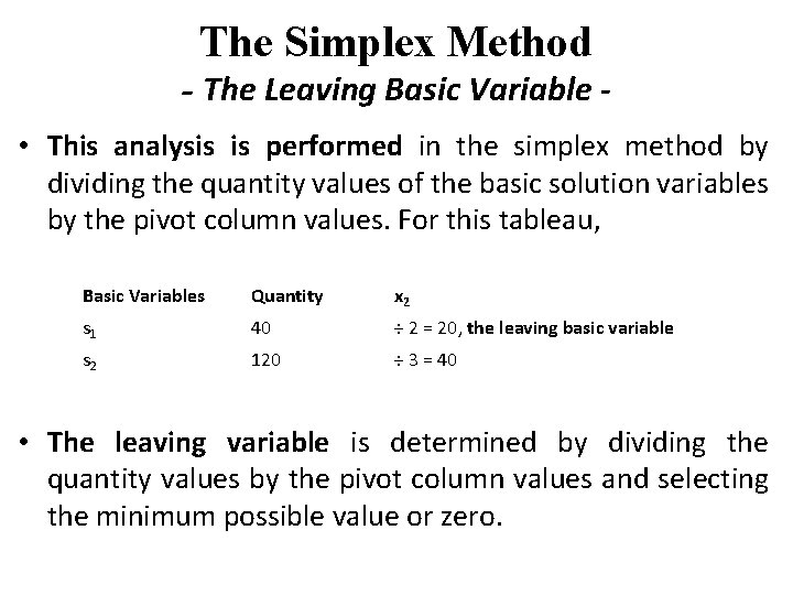
The Simplex Method - The Leaving Basic Variable • This analysis is performed in the simplex method by dividing the quantity values of the basic solution variables by the pivot column values. For this tableau, Basic Variables Quantity x 2 s 1 40 ÷ 2 = 20, the leaving basic variable s 2 120 ÷ 3 = 40 • The leaving variable is determined by dividing the quantity values by the pivot column values and selecting the minimum possible value or zero.

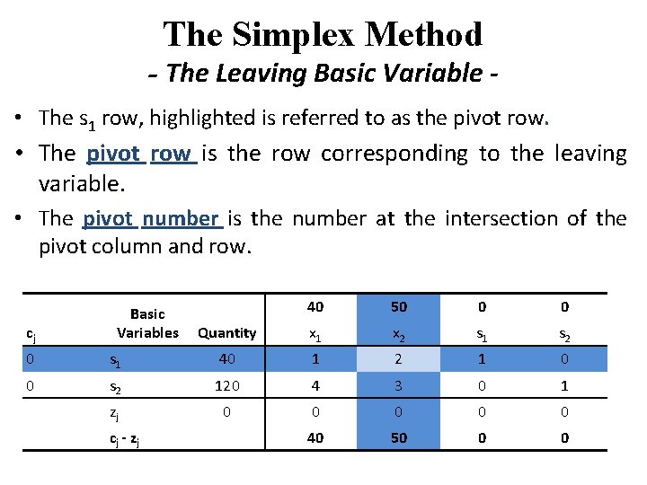
The Simplex Method - The Leaving Basic Variable • The s 1 row, highlighted is referred to as the pivot row. • The pivot row is the row corresponding to the leaving variable. • The pivot number is the number at the intersection of the pivot column and row. cj Basic Variables 40 50 0 0 Quantity x 1 x 2 s 1 s 2 0 s 1 40 1 2 1 0 0 s 2 120 4 3 0 1 zj 0 0 0 cj - zj 40 50 0 0

LINEAR PROGRAMMING THE SIMPLEX METHOD Developing a New Tableau

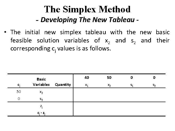
The Simplex Method - Developing The New Tableau • The initial new simplex tableau with the new basic feasible solution variables of x 2 and s 2 and their corresponding cj values is as follows. cj Basic Variables 50 x 2 0 s 2 zj cj - zj Quantity 40 50 0 0 x 1 x 2 s 1 s 2

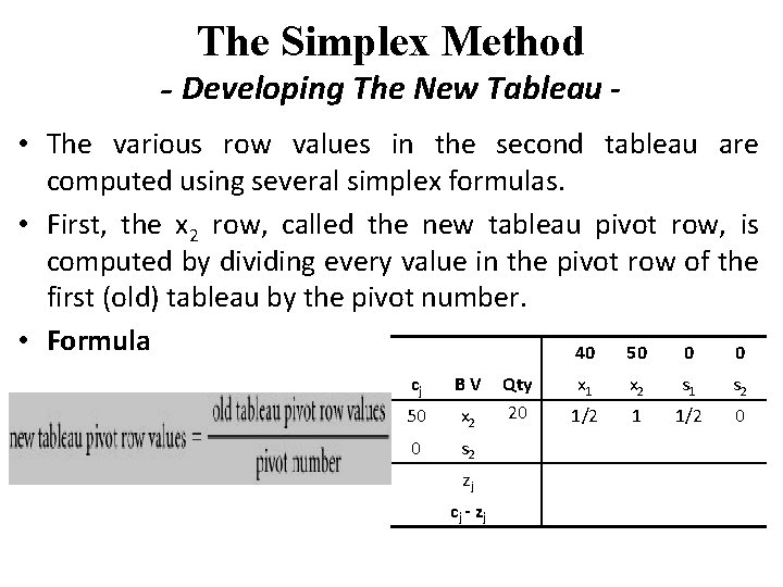
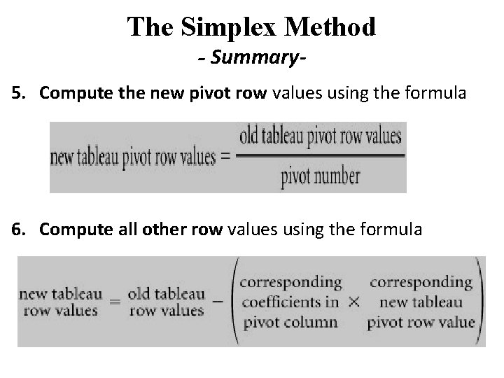
The Simplex Method - Developing The New Tableau • The various row values in the second tableau are computed using several simplex formulas. • First, the x 2 row, called the new tableau pivot row, is computed by dividing every value in the pivot row of the first (old) tableau by the pivot number. • Formula 40 50 0 0 cj B V 50 x 2 0 s 2 zj cj - zj Qty 20 x 1 x 2 s 1 s 2 1/2 1 1/2 0

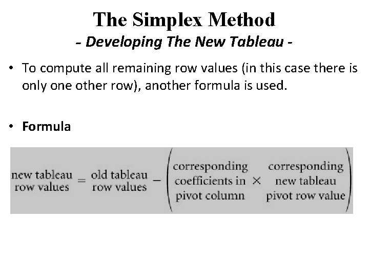
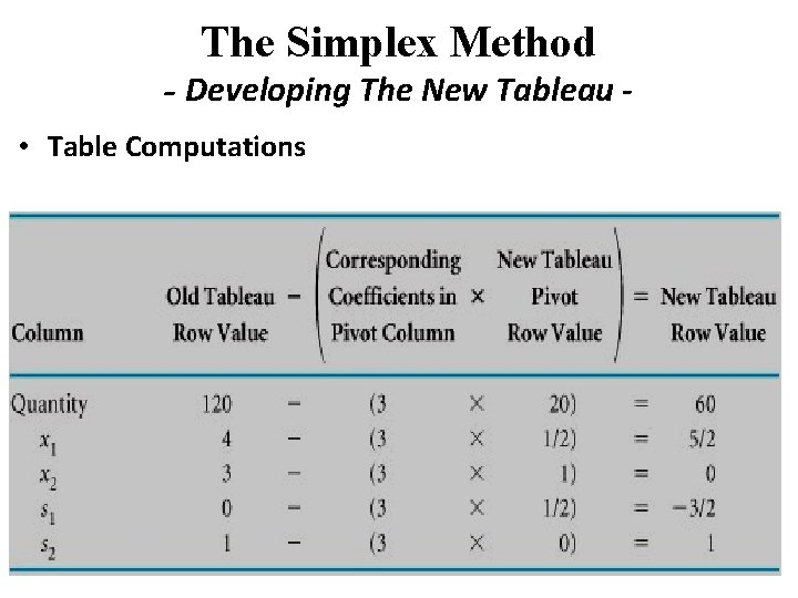
The Simplex Method - Developing The New Tableau • To compute all remaining row values (in this case there is only one other row), another formula is used. • Formula

The Simplex Method - Developing The New Tableau • Table Computations

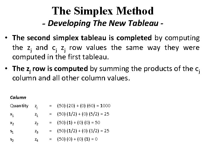
The Simplex Method - Developing The New Tableau • The second simplex tableau is completed by computing the zj and cj zj row values the same way they were computed in the first tableau. • The zj row is computed by summing the products of the cj column and all other column values. Column Quantity zj = (50) (20) + (0) (60) = 1000 x 1 z 1 = (50) (1/2) + (0) (5/2) = 25 x 2 z 2 = (50) (1) + (0) = 50 s 1 z 3 = (50) (1/2) + (0) (3/2) = 25 s 2 z 4 = (50) (0) + (0) (1) = 0

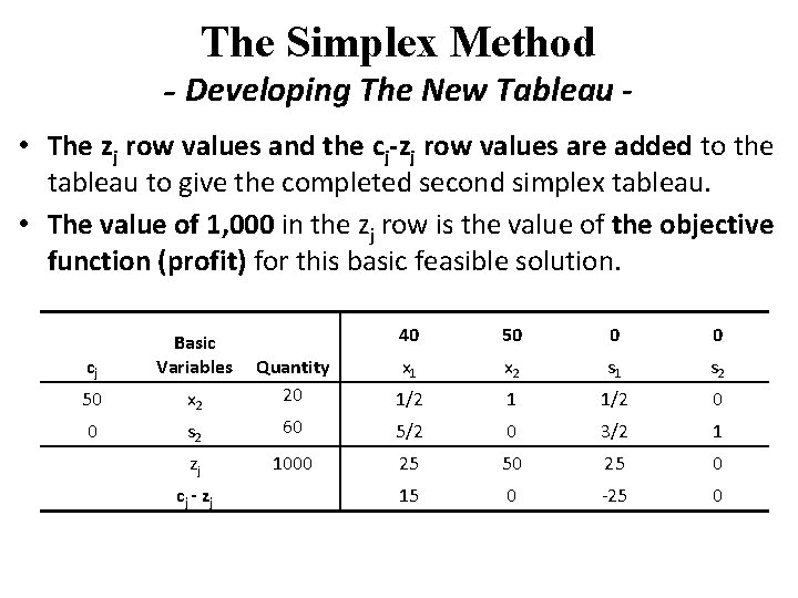
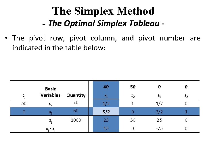
The Simplex Method - Developing The New Tableau • The zj row values and the cj-zj row values are added to the tableau to give the completed second simplex tableau. • The value of 1, 000 in the zj row is the value of the objective function (profit) for this basic feasible solution. cj Basic Variables 50 40 50 0 0 x 1 x 2 s 1 s 2 x 2 Quantity 20 1/2 1 1/2 0 0 s 2 60 5/2 0 3/2 1 zj 1000 25 50 25 0 cj - zj 15 0 -25 0

LINEAR PROGRAMMING THE SIMPLEX METHOD The Optimal Simplex Tableau

The Simplex Method - The Optimal Simplex Tableau • The steps that we followed to derive the second simplex tableau are repeated to develop the third tableau. • First, the pivot column or entering basic variable is determined. • Because 15 in the cj-zj row represents the greatest positive net increase in profit, x 1 becomes the entering nonbasic variable. • Dividing the pivot column values into the values in the quantity column indicates that s 2 is the leaving basic variable and corresponds to the pivot row.

The Simplex Method - The Optimal Simplex Tableau • The pivot row, pivot column, and pivot number are indicated in the table below: cj Basic Variables 50 40 50 0 0 x 1 x 2 s 1 s 2 x 2 Quantity 20 1/2 1 1/2 0 0 s 2 60 5/2 0 3/2 1 zj 1000 25 50 25 0 cj - zj 15 0 -25 0

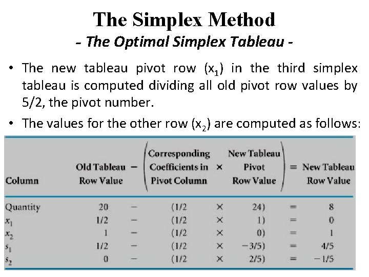
The Simplex Method - The Optimal Simplex Tableau • The new tableau pivot row (x 1) in the third simplex tableau is computed dividing all old pivot row values by 5/2, the pivot number. • The values for the other row (x 2) are computed as follows:

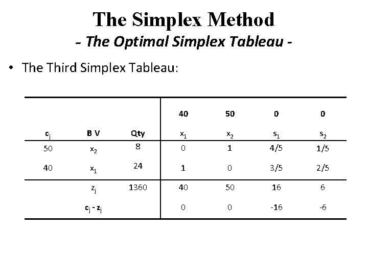
The Simplex Method - The Optimal Simplex Tableau • The Third Simplex Tableau: 40 50 0 0 x 1 x 2 s 1 s 2 0 1 4/5 1/5 cj B V 50 x 2 Qty 8 40 x 1 24 1 0 3/5 2/5 zj 1360 40 50 16 6 cj - zj 0 0 -16 -6

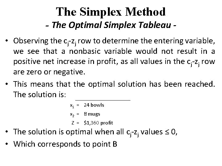
The Simplex Method - The Optimal Simplex Tableau • Observing the cj-zj row to determine the entering variable, we see that a nonbasic variable would not result in a positive net increase in profit, as all values in the cj-zj row are zero or negative. • This means that the optimal solution has been reached. The solution is: x 1 = 24 bowls x 2 = 8 mugs Z = $1, 360 profit • The solution is optimal when all cj-zj values ≤ 0, • Which corresponds to point B

LINEAR PROGRAMMING THE SIMPLEX METHOD Summary

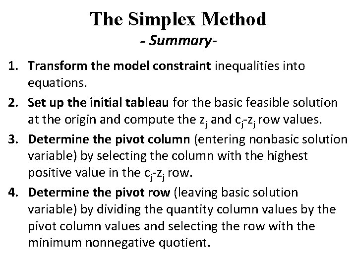
The Simplex Method - Summary 1. Transform the model constraint inequalities into equations. 2. Set up the initial tableau for the basic feasible solution at the origin and compute the zj and cj-zj row values. 3. Determine the pivot column (entering nonbasic solution variable) by selecting the column with the highest positive value in the cj-zj row. 4. Determine the pivot row (leaving basic solution variable) by dividing the quantity column values by the pivot column values and selecting the row with the minimum nonnegative quotient.

The Simplex Method - Summary 5. Compute the new pivot row values using the formula 6. Compute all other row values using the formula

The Simplex Method - Summary 7. Compute the new zj and cj-zj rows. 8. Determine whether or not the new solution is optimal by checking the cj-zj row. • • If all cj-zj row values are zero or negative, the solution is optimal. If a positive value exists, return to step 3 and repeat the simplex steps