Integer Programming m m Linear Programming Simplex method

Integer Programming m m Linear Programming (Simplex method) Integer Programming (Branch & Bound method) · Lasdon, L. S: Optimization Theory for Large Systems, Mac. Millan, 1970 (Section 1. 2) · CPLEX Manual · Cornuejols, G. , Trick, M. A. , and Saltzman, M. J. : A Tutorial on Integer Programming, Summer 1995, http: //mat. gsia. cmu. edu/orclass/integer. html Michał Pióro 1

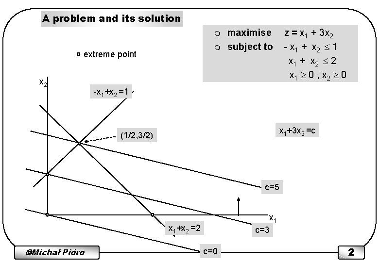
A problem and its solution m m extreme point x 2 maximise subject to z = x 1 + 3 x 2 - x 1 + x 2 1 x 1 + x 2 2 x 1 0 , x 2 0 -x 1+x 2 =1 x 1+3 x 2 =c (1/2, 3/2) c=5 x 1 c=3 x 1+x 2 =2 Michał Pióro c=0 2

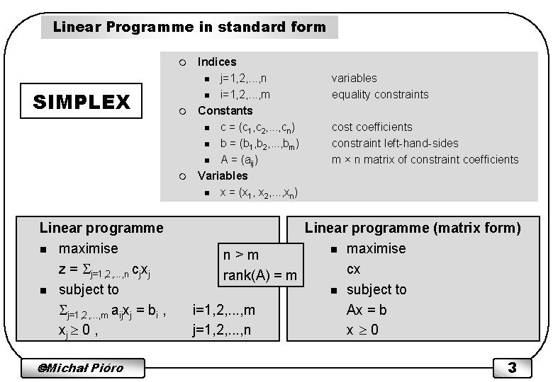
Linear Programme in standard form m SIMPLEX m m Linear programme n maximise z = j=1, 2, . . . , n cjxj n subject to j=1, 2, . . . , m aijxj = bi , xj 0 , Michał Pióro Indices n j=1, 2, . . . , n n i=1, 2, . . . , m Constants n c = (c 1, c 2, . . . , cn) n b = (b 1, b 2, . . . , bm) n A = (aij) Variables n x = (x 1, x 2, . . . , xn) variables equality constraints cost coefficients constraint left-hand-sides m × n matrix of constraint coefficients Linear programme (matrix form) n maximise n>m cx rank(A) = m n subject to i=1, 2, . . . , m Ax = b j=1, 2, . . . , n x 0 3

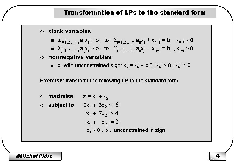
Transformation of LPs to the standard form m m slack variables n j=1, 2, . . . , m aijxj bi to j=1, 2, . . . , m aijxj + xn+i = bi , xn+i 0 n j=1, 2, . . . , m aijxj bi to j=1, 2, . . . , m aijxj - xn+i = bi , xn+i 0 nonnegative variables n xk with unconstrained sign: xk = xk - xk , xk 0 Exercise: transform the following LP to the standard form m maximise z = x 1 + x 2 m subject to 2 x 1 + 3 x 2 6 x 1 + 7 x 2 4 x 1 + x 2 = 3 x 1 0 , x 2 unconstrained in sign Michał Pióro 4

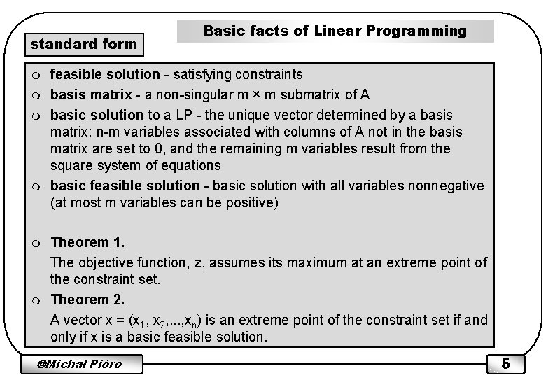
standard form m m m Basic facts of Linear Programming feasible solution - satisfying constraints basis matrix - a non-singular m × m submatrix of A basic solution to a LP - the unique vector determined by a basis matrix: n-m variables associated with columns of A not in the basis matrix are set to 0, and the remaining m variables result from the square system of equations basic feasible solution - basic solution with all variables nonnegative (at most m variables can be positive) Theorem 1. The objective function, z, assumes its maximum at an extreme point of the constraint set. Theorem 2. A vector x = (x 1, x 2, . . . , xn) is an extreme point of the constraint set if and only if x is a basic feasible solution. Michał Pióro 5

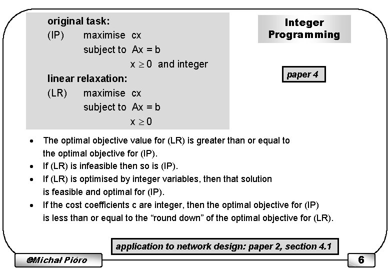
original task: (IP) maximise cx subject to Ax = b x 0 and integer linear relaxation: (LR) maximise cx subject to Ax = b x 0 · · Integer Programming paper 4 The optimal objective value for (LR) is greater than or equal to the optimal objective for (IP). If (LR) is infeasible then so is (IP). If (LR) is optimised by integer variables, then that solution is feasible and optimal for (IP). If the cost coefficients c are integer, then the optimal objective for (IP) is less than or equal to the “round down” of the optimal objective for (LR). application to network design: paper 2, section 4. 1 Michał Pióro 6

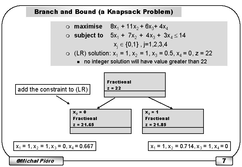
Branch and Bound (a Knapsack Problem) m maximise subject to 8 x 1 + 11 x 2 + 6 x 3+ 4 x 4 5 x 1 + 7 x 2 + 4 x 3 + 3 x 4 14 xj {0, 1} , j=1, 2, 3, 4 (LR) solution: x 1 = 1, x 2 = 1, x 3 = 0. 5, x 4 = 0, z = 22 n no integer solution will have value greater than 22 add the constraint to (LR) x 3 = 0 Fractional z = 21. 65 x 1 = 1, x 2 = 1, x 3 = 0, x 4 = 0. 667 Michał Pióro Fractional z = 22 x 3 = 1 Fractional z = 21. 85 x 1 = 1, x 2 = 0. 714, x 3 = 1, x 4 = 0 7

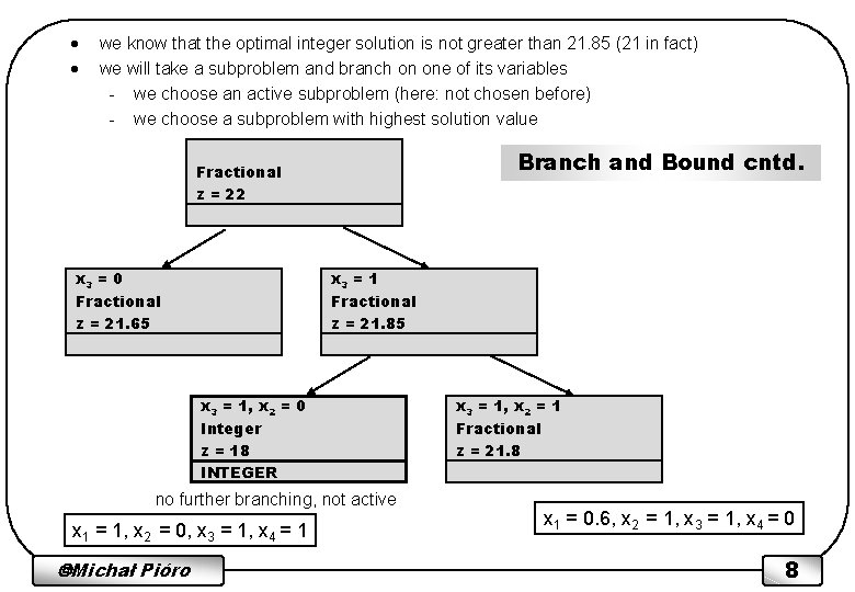
· · we know that the optimal integer solution is not greater than 21. 85 (21 in fact) we will take a subproblem and branch on one of its variables - we choose an active subproblem (here: not chosen before) - we choose a subproblem with highest solution value Branch and Bound cntd. Fractional z = 22 x 3 = 0 Fractional z = 21. 65 x 3 = 1 Fractional z = 21. 85 x 3 = 1, x 2 = 0 Integer z = 18 INTEGER no further branching, not active x 1 = 1, x 2 = 0, x 3 = 1, x 4 = 1 Michał Pióro x 3 = 1, x 2 = 1 Fractional z = 21. 8 x 1 = 0. 6, x 2 = 1, x 3 = 1, x 4 = 0 8

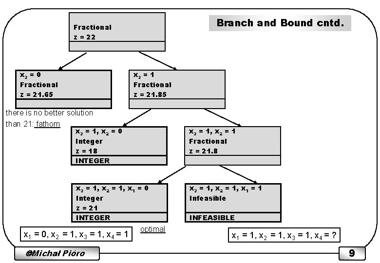
Branch and Bound cntd. Fractional z = 22 x 3 = 0 Fractional z = 21. 65 x 3 = 1 Fractional z = 21. 85 there is no better solution than 21: fathom x 3 = 1, x 2 = 0 Integer z = 18 INTEGER x 3 = 1, x 2 = 1 Fractional z = 21. 8 x 3 = 1, x 2 = 1, x 1 = 0 Integer z = 21 INTEGER x 3 = 1, x 2 = 1, x 1 = 1 Infeasible x 1 = 0, x 2 = 1, x 3 = 1, x 4 = 1 Michał Pióro optimal INFEASIBLE x 1 = 1, x 2 = 1, x 3 = 1, x 4 = ? 9

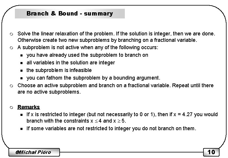
Branch & Bound - summary m m Solve the linear relaxation of the problem. If the solution is integer, then we are done. Otherwise create two new subproblems by branching on a fractional variable. A subproblem is not active when any of the following occurs: n you have already used the subproblem to branch on n all variables in the solution are integer n the subproblem is infeasible n you can fathom the subproblem by a bounding argument. Choose an active subproblem and branch on a fractional variable. Repeat until there are no active subproblems. Remarks n If x is restricted to integer (but not necessarily to 0 or 1), then if x = 4. 27 you would branch with the constraints x 4 and x 5. n If some variables are not restricted to integer you do not branch on them. Michał Pióro 10

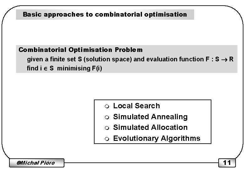
Basic approaches to combinatorial optimisation Combinatorial Optimisation Problem given a finite set S (solution space) and evaluation function F : S R find i S minimising F(i) m m Michał Pióro Local Search Simulated Annealing Simulated Allocation Evolutionary Algorithms 11

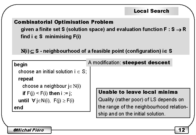
Local Search Combinatorial Optimisation Problem given a finite set S (solution space) and evaluation function F : S R find i S minimising F(i) N(i) S - neighbourhood of a feasible point (configuration) i S A modification: steepest descent begin choose an initial solution i S; repeat choose a neighbour j N(i) Unable to leave local minima if F(j) < F(i) then i : = j; Quality (rather poor) of LS depends on until j N(i), F(j) F(i) the range of the neighbourhood relationend ship and on the initial solution. Michał Pióro 12

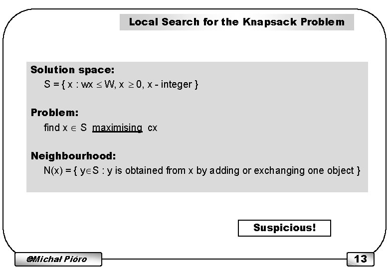
Local Search for the Knapsack Problem Solution space: S = { x : wx W, x 0, x - integer } Problem: find x S maximising cx Neighbourhood: N(x) = { y S : y is obtained from x by adding or exchanging one object } Suspicious! Michał Pióro 13

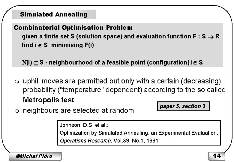
Simulated Annealing Combinatorial Optimisation Problem given a finite set S (solution space) and evaluation function F : S R find i S minimising F(i) N(i) S - neighbourhood of a feasible point (configuration) i S m m uphill moves are permitted but only with a certain (decreasing) probability (“temperature” dependent) according to the so called Metropolis test paper 5, section 3 neighbours are selected at random Johnson, D. S. et al. : Optimization by Simulated Annealing: an Experimental Evaluation, Operations Research, Vol. 39, No. 1, 1991 Michał Pióro 14

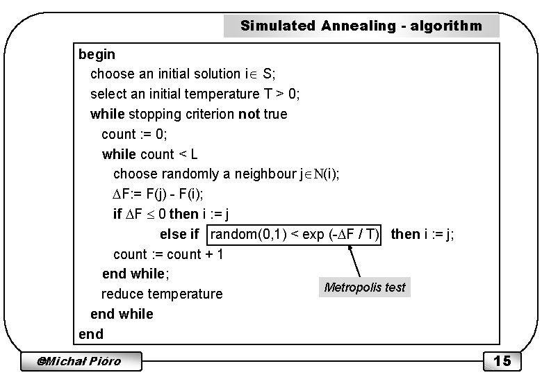
Simulated Annealing - algorithm begin choose an initial solution i S; select an initial temperature T > 0; while stopping criterion not true count : = 0; while count < L choose randomly a neighbour j N(i); F: = F(j) - F(i); if F 0 then i : = j else if random(0, 1) < exp (- F / T) then i : = j; count : = count + 1 end while; Metropolis test reduce temperature end while end Michał Pióro 15

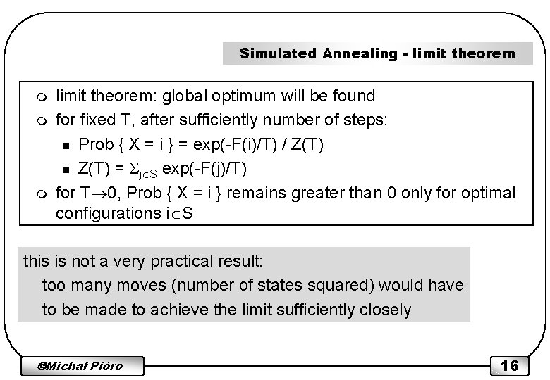
Simulated Annealing - limit theorem m limit theorem: global optimum will be found for fixed T, after sufficiently number of steps: n Prob { X = i } = exp(-F(i)/T) / Z(T) n Z(T) = j S exp(-F(j)/T) for T 0, Prob { X = i } remains greater than 0 only for optimal configurations i S this is not a very practical result: too many moves (number of states squared) would have to be made to achieve the limit sufficiently closely Michał Pióro 16

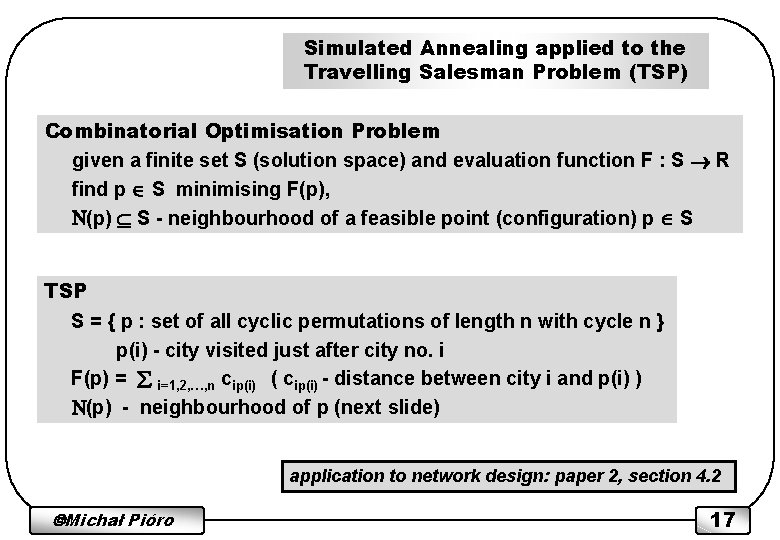
Simulated Annealing applied to the Travelling Salesman Problem (TSP) Combinatorial Optimisation Problem given a finite set S (solution space) and evaluation function F : S R find p S minimising F(p), N(p) S - neighbourhood of a feasible point (configuration) p S TSP S = { p : set of all cyclic permutations of length n with cycle n } p(i) - city visited just after city no. i F(p) = i=1, 2, …, n cip(i) ( cip(i) - distance between city i and p(i) ) N(p) - neighbourhood of p (next slide) application to network design: paper 2, section 4. 2 Michał Pióro 17

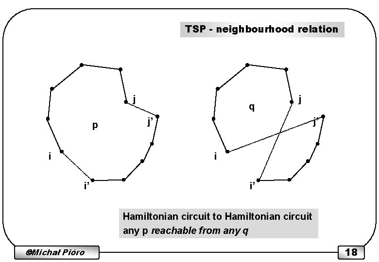
TSP - neighbourhood relation j p i q j j’ j’ i i’ i’ Hamiltonian circuit to Hamiltonian circuit any p reachable from any q Michał Pióro 18

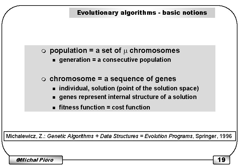
Evolutionary algorithms - basic notions m population = a set of chromosomes n m generation = a consecutive population chromosome = a sequence of genes n individual, solution (point of the solution space) genes represent internal structure of a solution n fitness function = cost function n Michalewicz, Z. : Genetic Algorithms + Data Structures = Evolution Programs, Springer, 1996 Michał Pióro 19

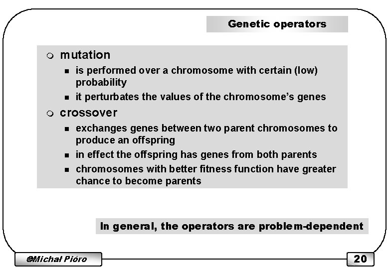
Genetic operators m mutation n n m is performed over a chromosome with certain (low) probability it perturbates the values of the chromosome’s genes crossover n n n exchanges genes between two parent chromosomes to produce an offspring in effect the offspring has genes from both parents chromosomes with better fitness function have greater chance to become parents In general, the operators are problem-dependent Michał Pióro 20

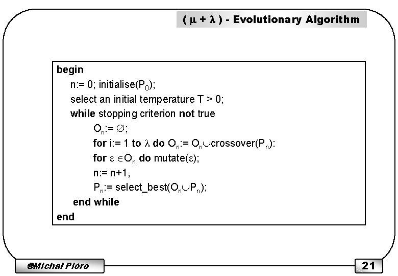
( + ) - Evolutionary Algorithm begin n: = 0; initialise(P 0); select an initial temperature T > 0; while stopping criterion not true On: = ; for i: = 1 to do On: = On crossover(Pn): for On do mutate( ); n: = n+1, Pn: = select_best(On Pn); end while end Michał Pióro 21

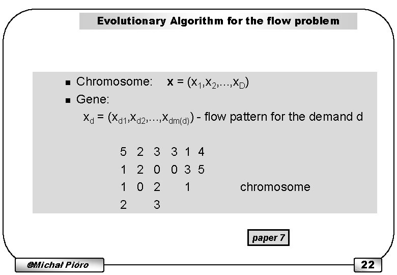
Evolutionary Algorithm for the flow problem n n Chromosome: x = (x 1, x 2, . . . , x. D) Gene: xd = (xd 1, xd 2, . . . , xdm(d)) - flow pattern for the demand d 5 2 3 3 1 4 1 2 0 0 3 5 1 0 2 1 2 3 chromosome paper 7 Michał Pióro 22

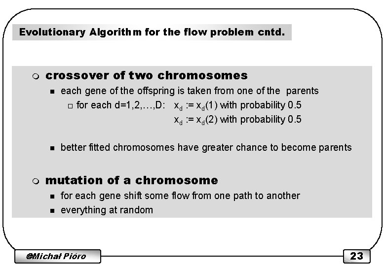
Evolutionary Algorithm for the flow problem cntd. m m crossover of two chromosomes n each gene of the offspring is taken from one of the parents o for each d=1, 2, …, D: xd : = xd(1) with probability 0. 5 xd : = xd(2) with probability 0. 5 n better fitted chromosomes have greater chance to become parents mutation of a chromosome n n for each gene shift some flow from one path to another everything at random Michał Pióro 23