The TwoPhase Simplex Method LI Xiaolei Preview n

The Two-Phase Simplex Method LI Xiao-lei

Preview n n When a basic feasible solution is not readily available, the two-phase simplex method may be used as an alternative to the big M method. In the two-phase simplex method, we add artificial variables to the same constraints as we did in big M method. Then we find a bfs to the original LP by solving the Phase I LP. In the Phase I LP, the objective function is to minimize the sum of all artificial variables. At the completion of Phase I, we reintroduce the original LP’s objective function and determine the optimal solution to the original LP.

The two-phase simplex method n Step 1 Modify the constraints so that the right-hand side of each constraint is nonnegative. This requires that each constraint with a negative right-hand side be multiplied through by -1. n Step 1’ Identify each constraint that is now an = or ≥ constraint. In step 3, we will add an the artificial variable to each of these constraints. n Step 2 Convert each inequality constraint to standard form. For ≤ constraint i, we add a slack variable si; For ≥ constraint i, we add an excess variable ei;

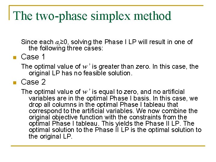
The two-phase simplex method n Step 4 For now, ignore the original LP’s objective function. Instead solve an LP whose objective function is min w’=(sum of all the artificial variables). This is called the Phase I LP. The act of solving the phase I LP will force the artificial variables to be zero.

The two-phase simplex method Since each ai≥ 0, solving the Phase I LP will result in one of the following three cases: n Case 1 The optimal value of w’ is greater than zero. In this case, the original LP has no feasible solution. n Case 2 The optimal value of w’ is equal to zero, and no artificial variables are in the optimal Phase I basis. In this case, we drop all columns in the optimal Phase I tableau that correspond to the artificial variables. We now combine the original objective function with the constraints from the optimal Phase I tableau. This yields the Phase II LP. The optimal solution to the Phase II LP is the optimal solution to the original LP.

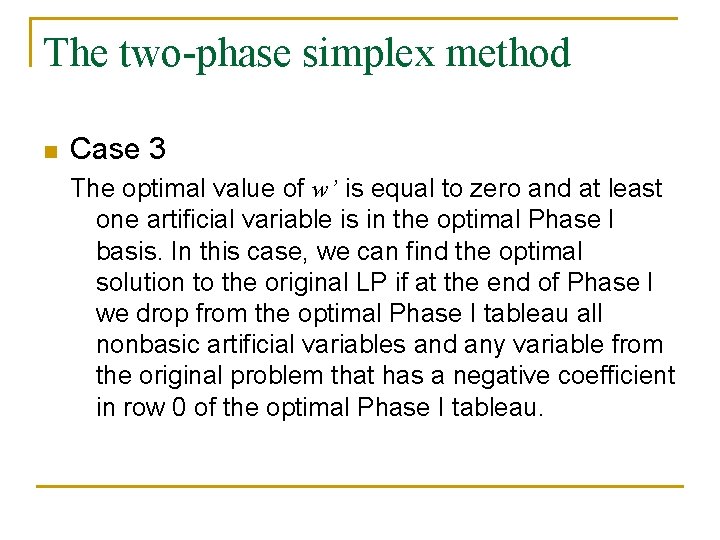
The two-phase simplex method n Case 3 The optimal value of w’ is equal to zero and at least one artificial variable is in the optimal Phase I basis. In this case, we can find the optimal solution to the original LP if at the end of Phase I we drop from the optimal Phase I tableau all nonbasic artificial variables and any variable from the original problem that has a negative coefficient in row 0 of the optimal Phase I tableau.

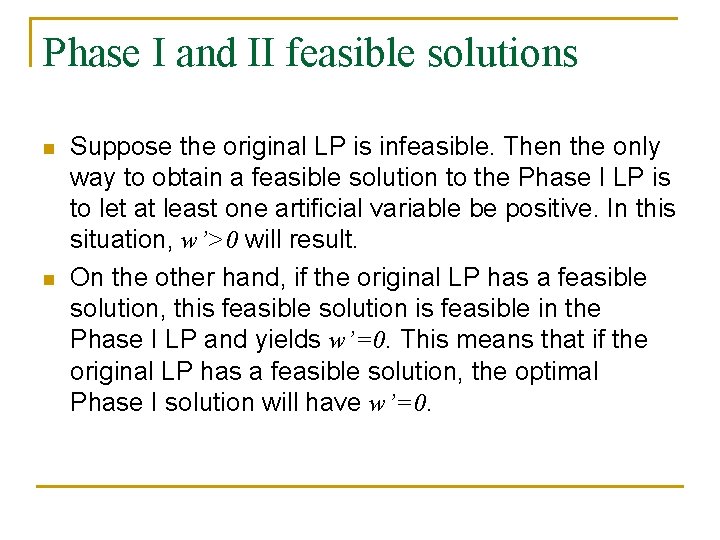
Phase I and II feasible solutions n n Suppose the original LP is infeasible. Then the only way to obtain a feasible solution to the Phase I LP is to let at least one artificial variable be positive. In this situation, w’>0 will result. On the other hand, if the original LP has a feasible solution, this feasible solution is feasible in the Phase I LP and yields w’=0. This means that if the original LP has a feasible solution, the optimal Phase I solution will have w’=0.

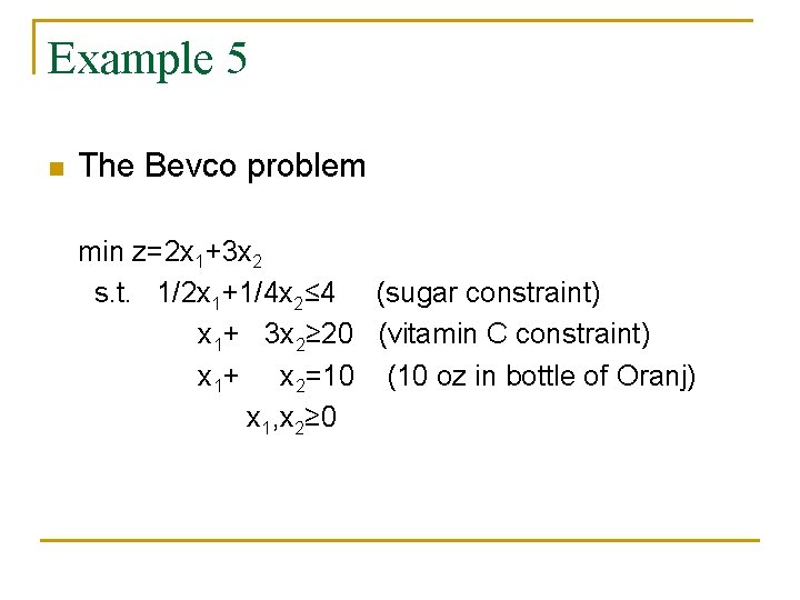
Example 5 n The Bevco problem min z=2 x 1+3 x 2 s. t. 1/2 x 1+1/4 x 2≤ 4 (sugar constraint) x 1+ 3 x 2≥ 20 (vitamin C constraint) x 1+ x 2=10 (10 oz in bottle of Oranj) x 1, x 2≥ 0

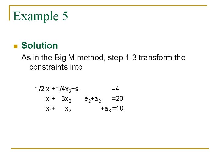
Example 5 n Solution As in the Big M method, step 1 -3 transform the constraints into 1/2 x 1+1/4 x 2+s 1 =4 x 1+ 3 x 2 -e 2+a 2 =20 x 1+ x 2 +a 3 =10

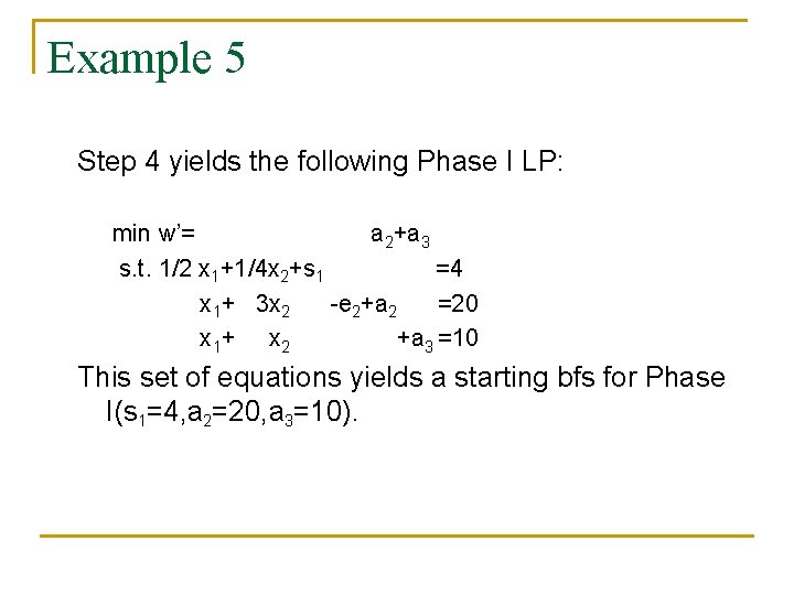
Example 5 Step 4 yields the following Phase I LP: min w’= a 2+a 3 s. t. 1/2 x 1+1/4 x 2+s 1 =4 x 1+ 3 x 2 -e 2+a 2 =20 x 1+ x 2 +a 3 =10 This set of equations yields a starting bfs for Phase I(s 1=4, a 2=20, a 3=10).

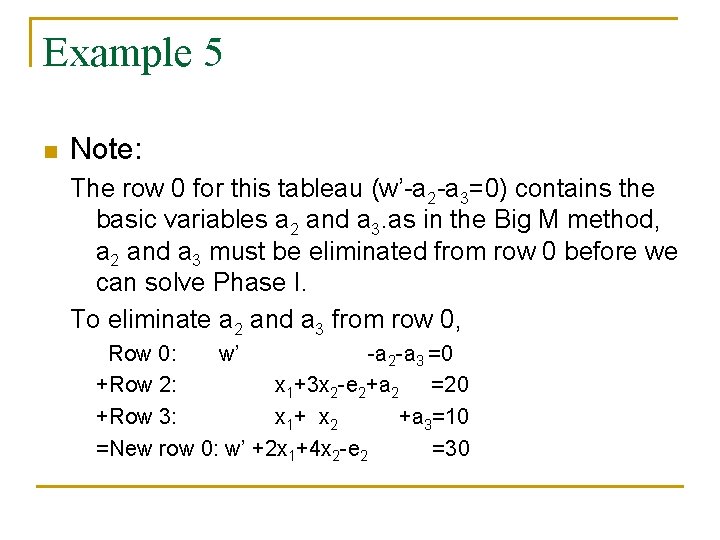
Example 5 n Note: The row 0 for this tableau (w’-a 2 -a 3=0) contains the basic variables a 2 and a 3. as in the Big M method, a 2 and a 3 must be eliminated from row 0 before we can solve Phase I. To eliminate a 2 and a 3 from row 0, Row 0: w’ -a 2 -a 3 =0 +Row 2: x 1+3 x 2 -e 2+a 2 =20 +Row 3: x 1+ x 2 +a 3=10 =New row 0: w’ +2 x 1+4 x 2 -e 2 =30

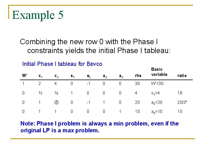
Example 5 Combining the new row 0 with the Phase I constraints yields the initial Phase I tableau: Initial Phase I tableau for Bevco W’ x 1 x 2 s 1 e 2 a 3 rhs Basic variable 1 2 4 0 -1 0 0 30 W’=30 0 ½ ¼ 1 0 0 0 4 s 1=4 16 0 1 ③ 0 -1 1 0 20 a 2=20 20/3* 0 1 1 0 0 0 1 10 a 3=10 10 ratio Note: Phase I problem is always a min problem, even if the original LP is a max problem.

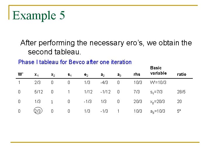
Example 5 After performing the necessary ero’s, we obtain the second tableau. Phase I tableau for Bevco after one iteration W’ x 1 x 2 s 1 e 2 a 3 rhs Basic variable 1 2/3 0 0 1/3 -4/3 0 10/3 W’=10/3 0 5/12 0 1 1/12 -1/12 0 7/3 s 1=7/3 28/5 0 1/3 1 0 -1/3 0 20/3 x 2=20/3 20 0 2/3 0 0 1/3 -1/3 1 10/3 a 3=10/3 5* ratio

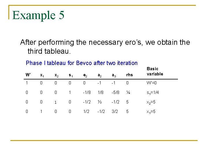
Example 5 After performing the necessary ero’s, we obtain the third tableau. Phase I tableau for Bevco after two iteration W’ x 1 x 2 s 1 e 2 a 3 rhs Basic variable 1 0 0 -1 -1 0 W’=0 0 1 -1/8 -5/8 ¼ s 1=1/4 0 0 1 0 -1/2 ½ -1/2 5 x 2=5 0 1 0 0 1/2 -1/2 3/2 5 x 1=5

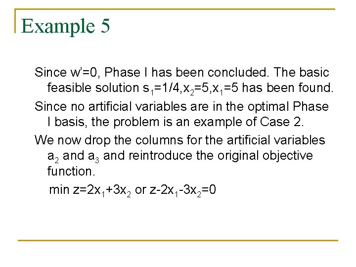
Example 5 Since w’=0, Phase I has been concluded. The basic feasible solution s 1=1/4, x 2=5, x 1=5 has been found. Since no artificial variables are in the optimal Phase I basis, the problem is an example of Case 2. We now drop the columns for the artificial variables a 2 and a 3 and reintroduce the original objective function. min z=2 x 1+3 x 2 or z-2 x 1 -3 x 2=0

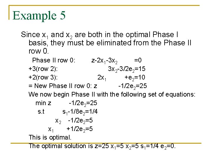
Example 5 Since x 1 and x 2 are both in the optimal Phase I basis, they must be eliminated from the Phase II row 0: z-2 x 1 -3 x 2 =0 +3(row 2): 3 x 2 -3/2 e 2=15 +2(row 3): 2 x 1 +e 2=10 = New Phase II row 0: z -1/2 e 2=25 We now begin Phase II with the following set of equations: min z -1/2 e 2=25 s. t s 1 -1/8 e 2=1/4 x 2 -1/2 e 2=5 x 1 +1/2 e 2=5 This is optimal. The optimal solution is z=25 x 1=5 x 2=5 s 1=1/4 e 2=0.

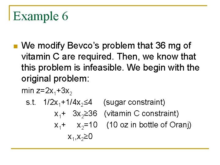
Example 6 n We modify Bevco’s problem that 36 mg of vitamin C are required. Then, we know that this problem is infeasible. We begin with the original problem: min z=2 x 1+3 x 2 s. t. 1/2 x 1+1/4 x 2≤ 4 (sugar constraint) x 1+ 3 x 2≥ 36 (vitamin C constraint) x 1+ x 2=10 (10 oz in bottle of Oranj) x 1, x 2≥ 0

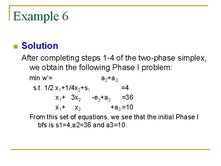
Example 6 n Solution After completing steps 1 -4 of the two-phase simplex, we obtain the following Phase I problem: min w’= a 2+a 3 s. t. 1/2 x 1+1/4 x 2+s 1 =4 x 1+ 3 x 2 -e 2+a 2 =36 x 1+ x 2 +a 3 =10 From this set of equations, we see that the initial Phase I bfs is s 1=4, a 2=36 and a 3=10.

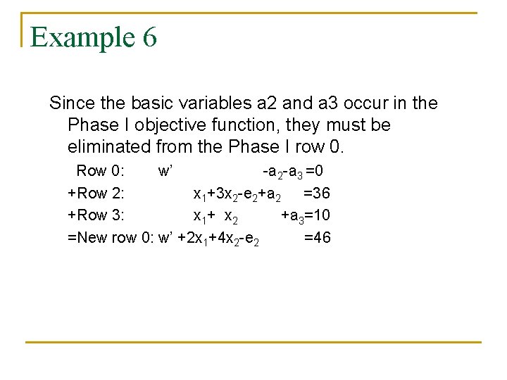
Example 6 Since the basic variables a 2 and a 3 occur in the Phase I objective function, they must be eliminated from the Phase I row 0. Row 0: w’ -a 2 -a 3 =0 +Row 2: x 1+3 x 2 -e 2+a 2 =36 +Row 3: x 1+ x 2 +a 3=10 =New row 0: w’ +2 x 1+4 x 2 -e 2 =46

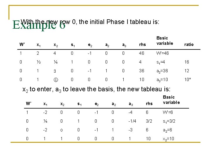
Example 6 With the new row 0, the initial Phase I tableau is: W’ x 1 x 2 s 1 e 2 a 3 rhs Basic variable 1 2 4 0 -1 0 0 46 W’=46 0 ½ ¼ 1 0 0 0 4 s 1=4 16 0 1 3 0 -1 1 0 36 a 2=36 12 0 1 ① 0 0 0 1 10 a 3=10 10* x 2 to enter, a 3 to leave the basis, the new tableau is: W’ x 1 x 2 s 1 e 2 a 3 rhs Basic variable 1 -2 0 0 -1 0 -4 6 W’=6 0 ¼ 0 1 0 0 -1/4 3/2 s 1=3/2 0 -2 0 0 -1 1 -3 6 a 2=6 0 1 1 0 0 0 1 10 x 2=10 ratio

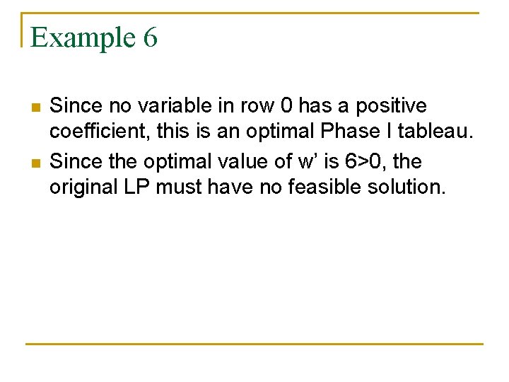
Example 6 n n Since no variable in row 0 has a positive coefficient, this is an optimal Phase I tableau. Since the optimal value of w’ is 6>0, the original LP must have no feasible solution.

Remarks n n As with the Big M method, the column for any artificial variable may be dropped from future tableaus as soon as the artificial variable leaves the basis. The Big M method and Phase I of the twpphase method make the same sequence of pivots. The two-phase method does not cause roundoff errors and other computational difficulties.