Longtime transients in open quantum systems Krzysztof Stefaski

Long-time transients in open quantum systems Krzysztof Stefański CM UMK Bydgoszcz/Toruń 44 th SMP, Toruń 2012

Transient behaviour – what does one mean? A behaviour of a dynamical system that is qualitatively different from its asymptotic (”eventual”) behaviour. Such a behaviour can be observed exclusively in dissipative systems!

Transient behaviours in classical open systems An example – transient chaos generated by maps with periodic attractors f : I → I, xn+1 = f(xn), e. g. Logistic maps, where f(x) = rx(1 -x)

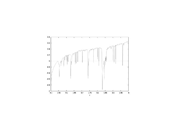
Bifurcation diagram for the family of Logistic maps

A vicinity of a period-5 window after 100 iterations

The same after 1000 iterations

1000000 Distribution of rambling times in a sample of 106 trajectories

Same in the semi-log scale

3 -D maps generating hyperchaotic trajectories:

A hyperchaotic attractor generated by an F 2 map

Disitribution of rambling times for a sample of 250 trajectories in the period-3 window (RT-axis unit: 106 iterations; the average is ca 0. 7 • 106(!)) [1]

Transient chaos in classical systems can be characterized by time evolution of the average finite-time estimates of Lyapunov exponent(s). For a typical set of trajectories one can observe a continuous decrease of the estimates and their convergence to the „true” Lyapunov exponents.

Time evolution of finite-time estimates of LE in a periodic window

Comparison of the model and nuericaly obtained time evolutions of AFTLE for a periodic window of the family of Logistic maps. [2]

And the quantum systems? 1. It may be a bit difficult to find a nondisputable equivalent of transient chaos. 2. However, one can look for various examples of quantum metastability.

A bit of algebra Fokker-Planck equation [3]: May be derived from the Langevine equation or Liouville-von Neumann equation

Expansion of P leads to the Schroedinger-like equation where [3]

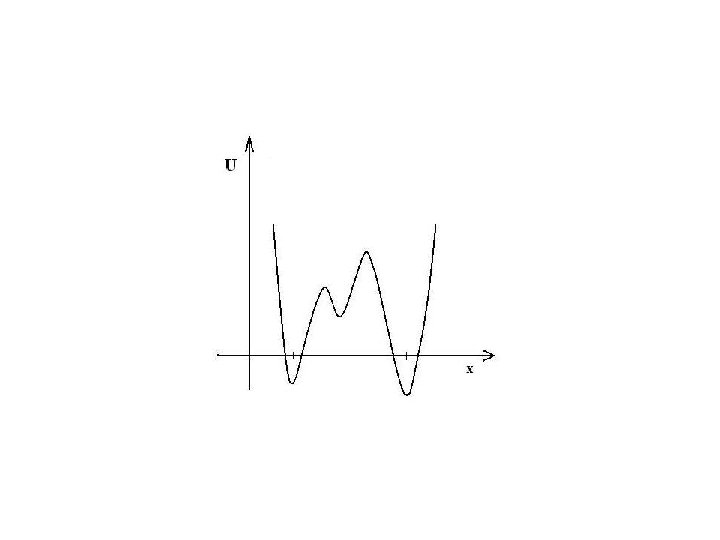
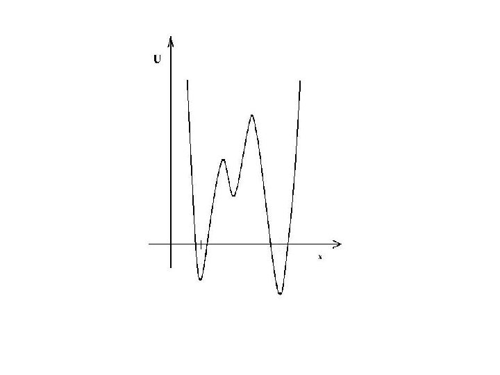
A schematic draft of the typical shape of the potential U in the case of bistability is shown below. Two wells with negative minima are separated by a barrier with an additional, positive-value minimum. Height of the barrier increases with the size of the system N (or, in general, with decrese of the amplitude of diffusion function q)

Such a potential implies that the two lowest eigenvalues λ 0 = 0, and λ 1 are close to each other, the closer, the higher the barrier (quasior near-degeneracy). The corresponding eigenfunctions are almost completely localized over the wells and differ mainly in that p 1 has a node:

Schematic plot of eigenfunctions p 0 for two various amplitudes of diffusion function q (or the size of the system N)

Same for the eigenfunctions p 1

Long time evolution of the system can be represented with the two eigenfunctions p 0 & p 1 only, since the remaining components of the expansion of P decay rapidly and do not count except for the very initial time interval Δτ defined by the formula Δτ = k/λ 2, where k follows from the required level of accuracy of the approximation: P(x, t) ≈ A 0χ(x)p 0(x) + A 1χ(x)p 1(x)exp(- λ 1 t).

Eigenfunction p 0 for the eigenvalue λ 0

Eigenfunction p 1 for the eigenvalue λ 1

For times fulfilling the double inequality: k/λ 2 < t ≪ 1/λ 1, instead of p 0 and p 1, shown above, one can use another pair of quasi-eigenfunctions p. L & p. R, that are shown below:

Pseudo-eigenfunction p. L

Pseudo-eigenfunction p. R

Two comments: 1. In the quantum Hamiltonian eigenproblems with a double-well potential one obtains almost identical eigenfunctions but their physical meaning is essentially different leaving n room for transients. 2. In the case of classical transient chaos trajectories while approaching the attractor have to ”tunnel” through a labyrinth-like ”pesudobarrier”.

Conclusions (? ) 1. Laser with saturable absorber (or dye laser) provides a simple model for quantum tunneling and, consequently, transient behavior in essentially quantum systems. 2. Large molecules (e. g. proteins) may be even more interesting and potentially important (though difficult) subjects for similar treatment and analysis.

Th. Y. f. Y. A.

Some references: [1] K. Stefański: Chaotic transients in multidimenional maps, Rep. Math. Phys. 44, 231 -240 (1999). [2] K. Stefański, K. Buszko, K. Piecyk: Transient chaos measurements using finite-time. Lyapunov exponents, Chaos 20, 033117 -13 (2010). [3] K. Stefański: Quantum description of a dye laser threshold region, Z. Phys. B 45, 351 -361 (1982).