Learning in Games Georgios Piliouras Games i e

Learning in Games Georgios Piliouras

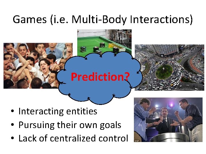
Games (i. e. Multi-Body Interactions) Prediction? • Interacting entities • Pursuing their own goals • Lack of centralized control

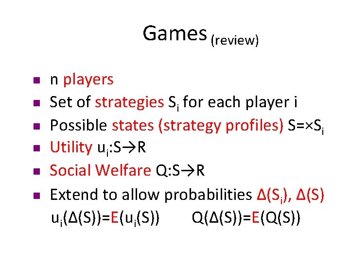
Games (review) n n n n players Set of strategies Si for each player i Possible states (strategy profiles) S=×Si Utility ui: S→R Social Welfare Q: S→R Extend to allow probabilities Δ(Si), Δ(S) ui(Δ(S))=E(ui(S)) Q(Δ(S))=E(Q(S))

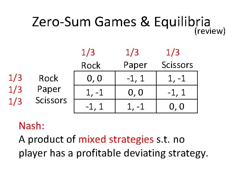
Zero-Sum Games & Equilibria (review) 1/3 1/3 Rock Paper Scissors 1/3 Rock 0, 0 1, -1 -1, 1 1/3 Paper -1, 1 0, 0 1, -1 1/3 Scissors 1, -1 -1, 1 0, 0 Nash: A product of mixed strategies s. t. no player has a profitable deviating strategy.

Why do we study Nash eq? § Nash eq. have a simple intuitive definition. § Nash eq. are applicable to all games. § In some classes of games, Nash eq. is reasonably good predictor of rational self -interested behavior (e. g. zero-sum games). § Even in general games, Nash eq. analysis seems like a natural, albeit optimistic, first step in understanding rational behavior.

Why is it optimistic? Nash eq. analysis presumes that agents can resolve issues regarding: § Convergence: Agent behavior will converge to a Nash. § Coordination: If there are many Nash eq, agents can coordinate on one of them. § Communication: Agents are fully aware of each other utilities/rationality. § Complexity: Computing a Nash can be hard even from a centralized perspective.

Today: Learning in Games Agent behavior is online learning algorithm/dynamic Input: Current state of environment/other agents (+ history) Output: Chosen (randomized) action Analyze the evolution of systems of coupled dynamics, as a way to predict interacting agent behavior. Advantages: Weaker assumptions. If dynamic converges Nash equilibrium (may not converge) Disadvantages: Harder to analyze

Today: Learning in Games Agent behavior is online learning algorithm/dynamic Input: Current state of environment/other agents (+ history) Output: Chosen (randomized) action Class 1: Best (Better) Response Dynamics Class 2: No-regret dynamics (e. g. Weighted Majority/Hedge dynamic)

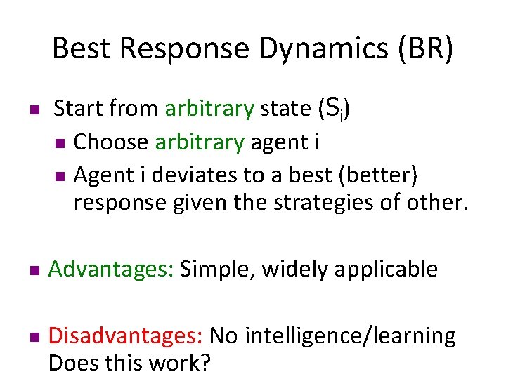
Best Response Dynamics (BR) n n n Start from arbitrary state (Si) n Choose arbitrary agent i n Agent i deviates to a best (better) response given the strategies of other. Advantages: Simple, widely applicable Disadvantages: No intelligence/learning Does this work?

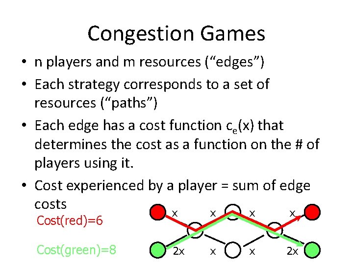
Congestion Games • n players and m resources (“edges”) • Each strategy corresponds to a set of resources (“paths”) • Each edge has a cost function ce(x) that determines the cost as a function on the # of players using it. • Cost experienced by a player = sum of edge costs x x Cost(red)=6 Cost(green)=8 2 x x x 2 x

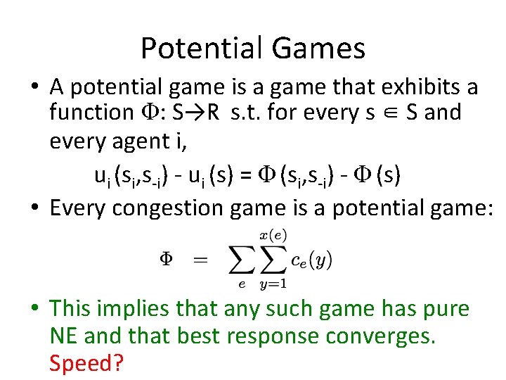
Potential Games • A potential game is a game that exhibits a function Φ: S→R s. t. for every s ∈ S and every agent i, ui (si, s-i) - ui (s) = Φ (si, s-i) - Φ (s) • Every congestion game is a potential game: • This implies that any such game has pure NE and that best response converges. Speed?

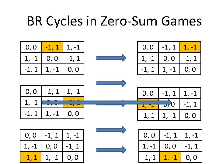
BR Cycles in Zero-Sum Games 0, 0 -1, 1 1, -1 1, -1 0, 0 -1, 1 -1, 1 1, -1 0, 0 0, 0 -1, 1 1, -1 0, 0 -1, 1 1, -1 0, 0

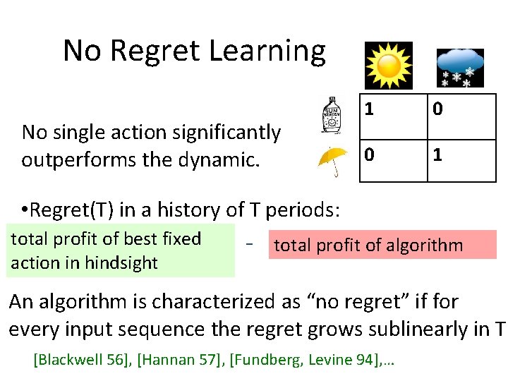
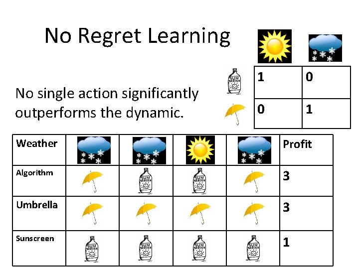
No Regret Learning No single action significantly outperforms the dynamic. 1 0 0 1 • Regret(T) in a history of T periods: total profit of best fixed action in hindsight - total profit of algorithm An algorithm is characterized as “no regret” if for every input sequence the regret grows sublinearly in T. [Blackwell 56], [Hannan 57], [Fundberg, Levine 94], …

No Regret Learning No single action significantly outperforms the dynamic. 1 0 0 1 Weather Profit Algorithm 3 Umbrella 3 Sunscreen 1

The Multiplicative Weights Algorithm a. k. a. Hedge a. k. a. Weighted Majority [Littlestone Warmuth ’ 94, Freund Schapire ‘ 99] • Pick s with probability proportional to (1 -ε)total(s), where total(s) denotes cumulative cost in all past periods. • Why is it regret minimizing? –Proof on the board.

No Regret and Equilibria Do no-regret algorithms converge to Nash equilibria in general games? Do no-regret algorithms converge to other equilibria in general games?

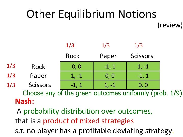
Other Equilibrium Notions 1/3 1/3 1/3 Rock Paper (review) 1/3 Scissors Rock Paper Scissors 0, 0 -1, 1 1, -1 0, 0 Choose any of the green outcomes uniformly (prob. 1/9) Nash: A probability distribution over outcomes, that is a product of mixed strategies s. t. no player has a profitable deviating strategy.

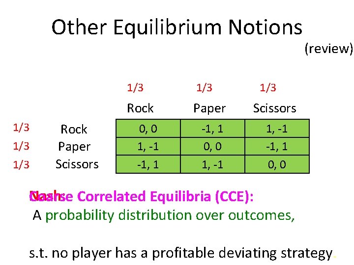
Other Equilibrium Notions 1/3 1/3 Rock Paper Scissors -1, 1 0, 0 1, -1 -1, 1 (review) 1/3 Nash: Coarse Correlated Equilibria (CCE): A probability distribution over outcomes, s. t. no player has a profitable deviating strategy.

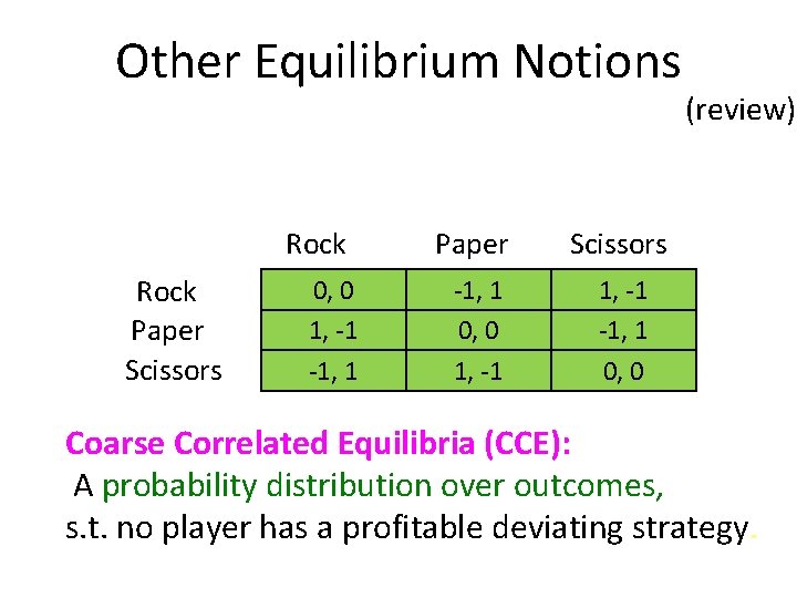
Other Equilibrium Notions Rock Paper Scissors 0, 0 1, -1 -1, 1 Paper Scissors -1, 1 0, 0 1, -1 -1, 1 0, 0 (review) Coarse Correlated Equilibria (CCE): A probability distribution over outcomes, s. t. no player has a profitable deviating strategy.

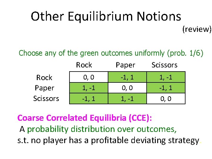
Other Equilibrium Notions (review) Choose any of the green outcomes uniformly (prob. 1/6) Rock Paper Scissors 0, 0 1, -1 -1, 1 Paper Scissors -1, 1 0, 0 1, -1 -1, 1 0, 0 Coarse Correlated Equilibria (CCE): A probability distribution over outcomes, s. t. no player has a profitable deviating strategy.

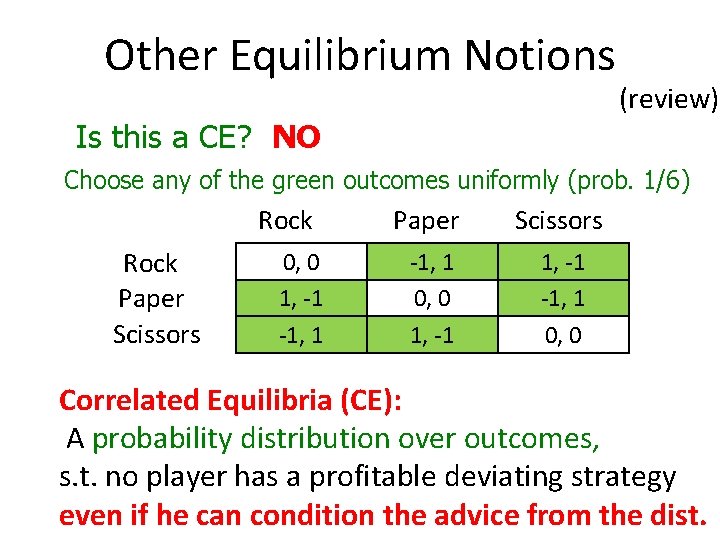
Other Equilibrium Notions (review) Is this a CE? NO Choose any of the green outcomes uniformly (prob. 1/6) Rock Paper Scissors 0, 0 1, -1 -1, 1 Paper Scissors -1, 1 0, 0 1, -1 -1, 1 0, 0 Correlated Equilibria (CE): A probability distribution over outcomes, s. t. no player has a profitable deviating strategy even if he can condition the advice from the dist.

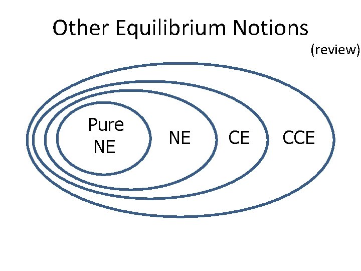
Other Equilibrium Notions Pure NE NE CE (review) CCE

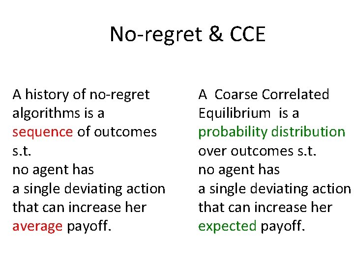
No-regret & CCE A history of no-regret algorithms is a sequence of outcomes s. t. no agent has a single deviating action that can increase her average payoff. A Coarse Correlated Equilibrium is a probability distribution over outcomes s. t. no agent has a single deviating action that can increase her expected payoff.

BREAK

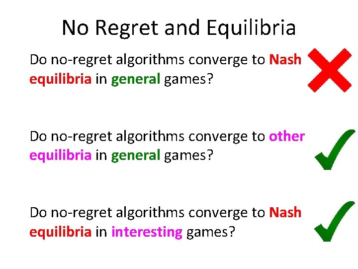
No Regret and Equilibria Do no-regret algorithms converge to Nash equilibria in general games? Do no-regret algorithms converge to other equilibria in general games? Do no-regret algorithms converge to Nash equilibria in interesting games?

CCE in Zero-Sum Games In general games, CCE ⊇ conv(NE) Why? In zero-sum games, CCE = conv(NE) Why? What does it imply for no-regret algs?

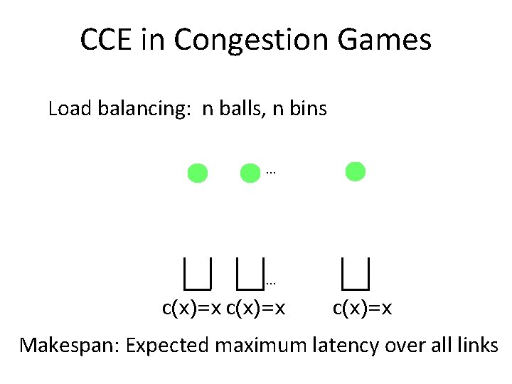
CCE in Congestion Games Load balancing: n balls, n bins … … c(x)=x Makespan: Expected maximum latency over all links

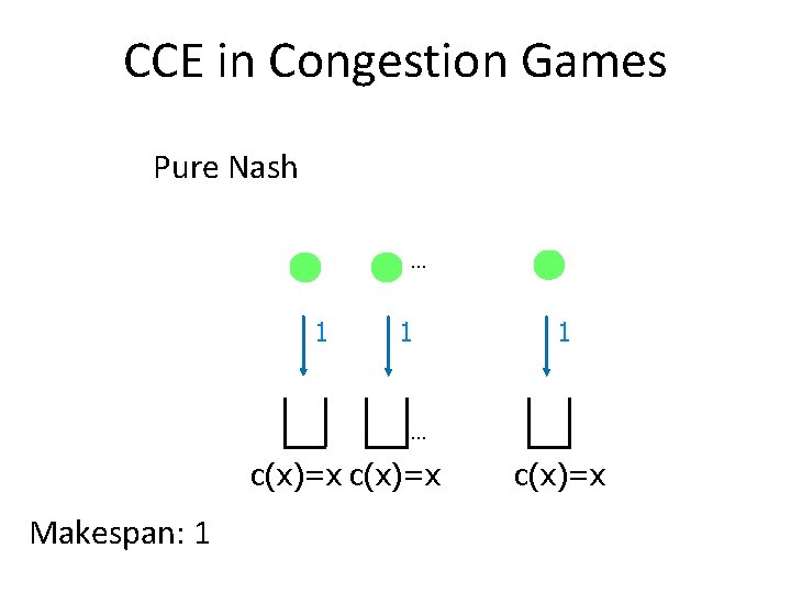
CCE in Congestion Games Pure Nash … 1 1 1 … c(x)=x Makespan: 1 c(x)=x

CCE in Congestion Games Mixed Nash [Koutsoupias, Mavronicolas, Spirakis ’ 02], [Czumaj, Vöcking ’ 02] … 1/n 1/n … c(x)=x Makespan: Θ(logn/loglogn) c(x)=x

CCE in Congestion Games [Blum, Hajiaghayi, Ligett, Roth ’ 08] Coarse Correlated Equilibria … … c(x)=x Makespan: Exponentially worse Ω(√n)

No-Regret Algs in Congestion Games Since worst case CCE can be reproduced by worst case no-regret algs, worst case no-regret algorithms do not converge to Nash equilibria in general.

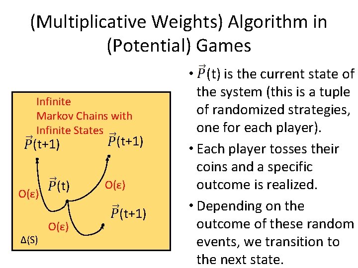
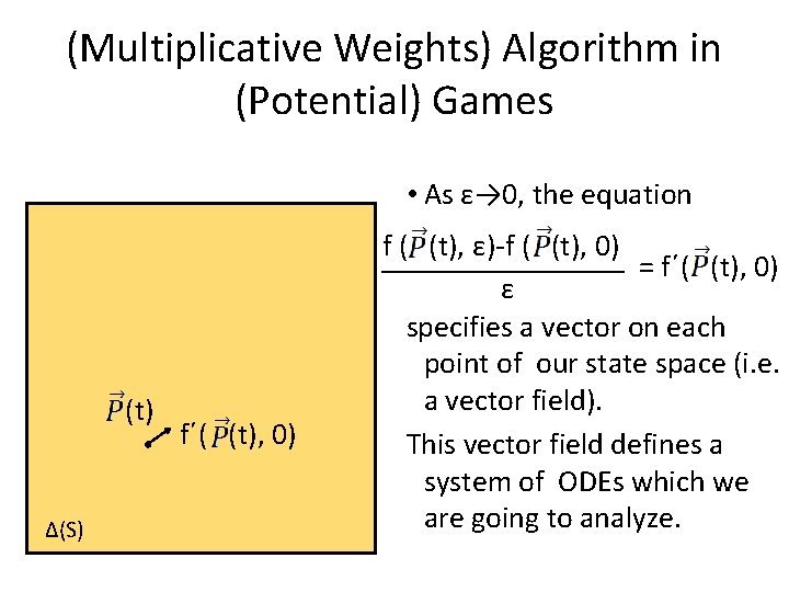
(Multiplicative Weights) Algorithm in (Potential) Games Infinite Markov Chains with Infinite States (t+1) O(ε) Δ(S) (t) O(ε) (t+1) • (t) is the current state of the system (this is a tuple of randomized strategies, one for each player). • Each player tosses their coins and a specific outcome is realized. • Depending on the outcome of these random events, we transition to the next state.

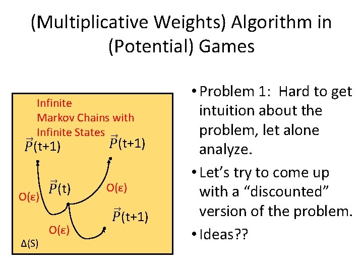
(Multiplicative Weights) Algorithm in (Potential) Games Infinite Markov Chains with Infinite States (t+1) O(ε) Δ(S) (t) O(ε) (t+1) • Problem 1: Hard to get intuition about the problem, let alone analyze. • Let’s try to come up with a “discounted” version of the problem. • Ideas? ?

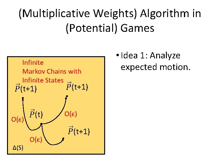
(Multiplicative Weights) Algorithm in (Potential) Games Infinite Markov Chains with Infinite States (t+1) O(ε) Δ(S) (t) O(ε) (t+1) • Idea 1: Analyze expected motion.

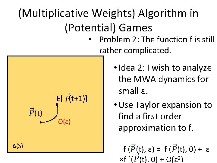
(Multiplicative Weights) Algorithm in (Potential) Games • Idea 1: Analyze expected motion. E[ (t+1)] (t) Δ(S) O(ε) • The system evolution is now deterministic. (i. e. there exists a function f, s. t. E[ (t+1)]= f ( (t), ε ) • I wish to analyze this function (e. g. find fixed points).

(Multiplicative Weights) Algorithm in (Potential) Games • Problem 2: The function f is still rather complicated. E[ (t+1)] (t) Δ(S) O(ε) • Idea 2: I wish to analyze the MWA dynamics for small ε. • Use Taylor expansion to find a first order approximation to f. f ( (t), ε) = f ( (t), 0) + ε ×f ´( (t), 0) + O(ε 2)

(Multiplicative Weights) Algorithm in (Potential) Games • As ε→ 0, the equation (t) Δ(S) f´( (t), 0) f ( (t), ε)-f ( (t), 0) = f´( (t), 0) ε specifies a vector on each point of our state space (i. e. a vector field). This vector field defines a system of ODEs which we are going to analyze.

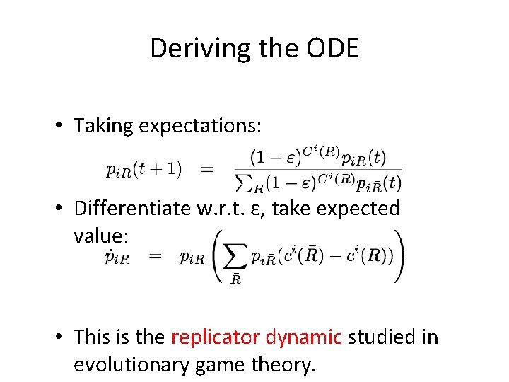
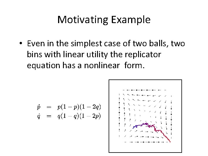
Deriving the ODE • Taking expectations: • Differentiate w. r. t. ε, take expected value: • This is the replicator dynamic studied in evolutionary game theory.

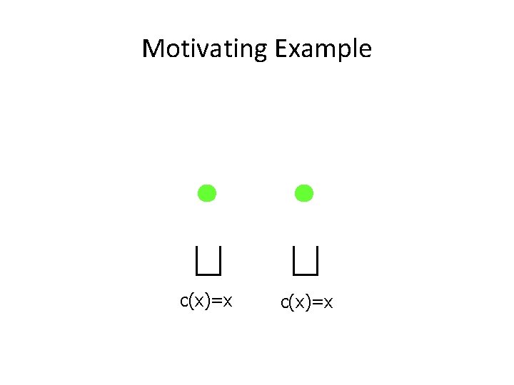
Motivating Example c(x)=x

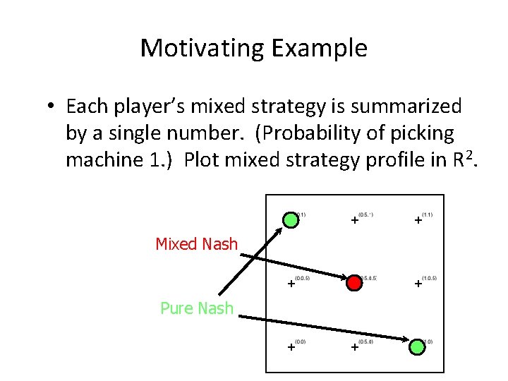
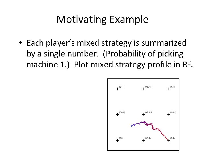
Motivating Example • Each player’s mixed strategy is summarized by a single number. (Probability of picking machine 1. ) Plot mixed strategy profile in R 2. Mixed Nash Pure Nash

Motivating Example • Each player’s mixed strategy is summarized by a single number. (Probability of picking machine 1. ) Plot mixed strategy profile in R 2.

Motivating Example • Even in the simplest case of two balls, two bins with linear utility the replicator equation has a nonlinear form.

The potential function • The congestion game has a potential function • Let Ψ=E[Φ]. A calculation yields • Hence Ψ decreases except when every player randomizes over paths of equal expected cost (i. e. is a Lyapunov function of the dynamics). [Monderer-Shapley ’ 96]. Analyzing the spectrum of the Jacobian shows that in “generic” congestion games only pure Nash are stable. [Kleinberg-Piliouras-Tardos ‘ 09]

BREAK 2 Can learning beat the BEST NASH by an arbitrary factor?

Cyclic Matching Pennies (Jordan’s game) [Jordan ’ 93] Nash Equilibrium H, T ½, ½ • H, T ½, ½ Profit of 1 if you mismatch opponent; 0 otherwise H, T ½, ½ Social Welfare of NE: 3/2

Cyclic Matching Pennies (Jordan’s game) [Jordan ’ 93] Best Response H, T Profit of 1 if you mismatch opponent; 0 otherwise Cycle H, T • • H, T Social Welfare of NE: 3/2 (H, H, T)

Cyclic Matching Pennies (Jordan’s game) [Jordan ’ 93] Best Response H, T Profit of 1 if you mismatch opponent; 0 otherwise Cycle H, T • • H, T Social Welfare of NE: 3/2 (H, H, T), (H, T, T)

Cyclic Matching Pennies (Jordan’s game) [Jordan ’ 93] Best Response H, T Profit of 1 if you mismatch opponent; 0 otherwise Cycle H, T • • H, T Social Welfare of NE: 3/2 (H, H, T), (H, T, H), (T, H, T), (H, H, T) Social Welfare: 2

Cyclic Matching Pennies (Jordan’s game) player i-1 [Jordan ’ 93] Best Response H, T player i Cycle H T H 0 1 T 1 0 payoff, i ∈ {0, 1, 2} H, T • • H, T Social Welfare of NE: 3/2 (H, H, T), (H, T, H), (T, H, T), (H, H, T) Social Welfare: 2

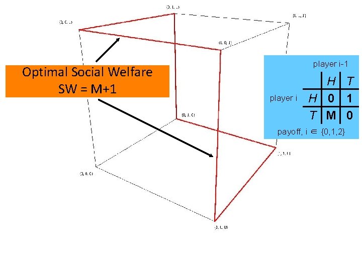
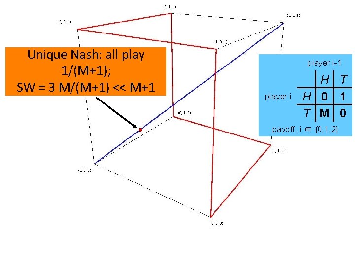
Asymmetric Cyclic Matching Pennies player i-1 [Jordan ’ 93] Best Response Cycle H, T 1/(M+1), M/(M+1) player i H T H 0 1 T M 0 payoff, i ∈ {0, 1, 2} H, T 1/(M+1), M/(M+1) • • H, T 1/(M+1), M/(M+1) Social Welfare of NE: 3 M/(M+1) < 3 (H, H, T), (H, T, H), (T, H, T), (H, H, T) Social Welfare:

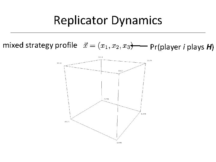
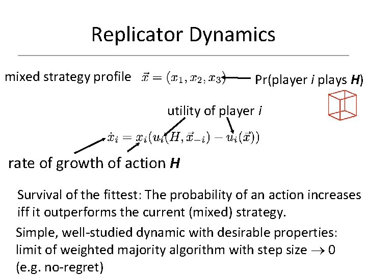
Replicator Dynamics mixed strategy profile Pr(player i plays H)

Replicator Dynamics mixed strategy profile Pr(player i plays H) utility of player i rate of growth of action H Survival of the fittest: The probability of an action increases iff it outperforms the current (mixed) strategy. Simple, well-studied dynamic with desirable properties: limit of weighted majority algorithm with step size 0 (e. g. no-regret)

Optimal Social Welfare SW = M+1 player i-1 player i H T H 0 1 T M 0 payoff, i ∈ {0, 1, 2}

Unique Nash: all play 1/(M+1); SW = 3 M/(M+1) << M+1 player i-1 player i H T H 0 1 T M 0 payoff, i ∈ {0, 1, 2}

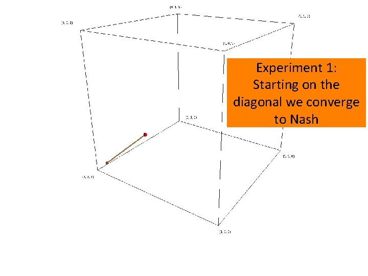
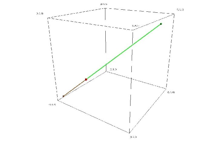
Experiment 1: Starting on the diagonal we converge to Nash

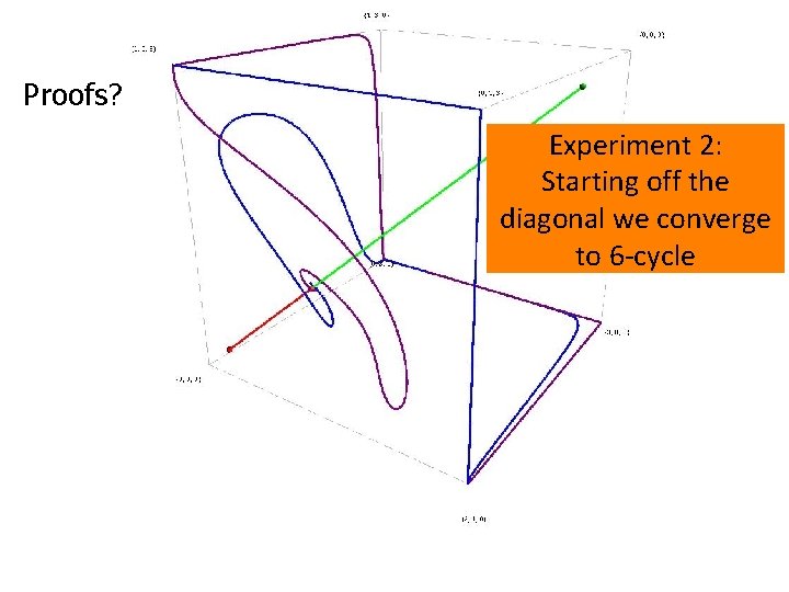
Proofs? Experiment 2: Starting off the diagonal we converge to 6 -cycle

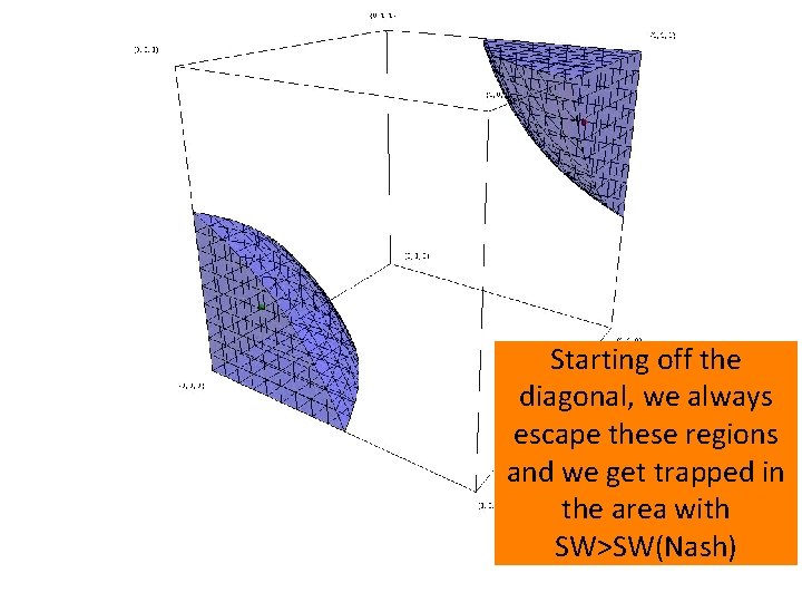
As M increases, the region where the SW is not a Lyapunov, increases as well.

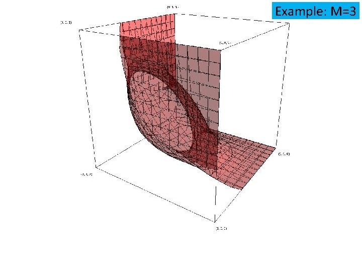
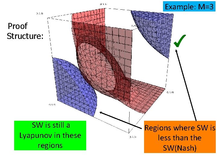
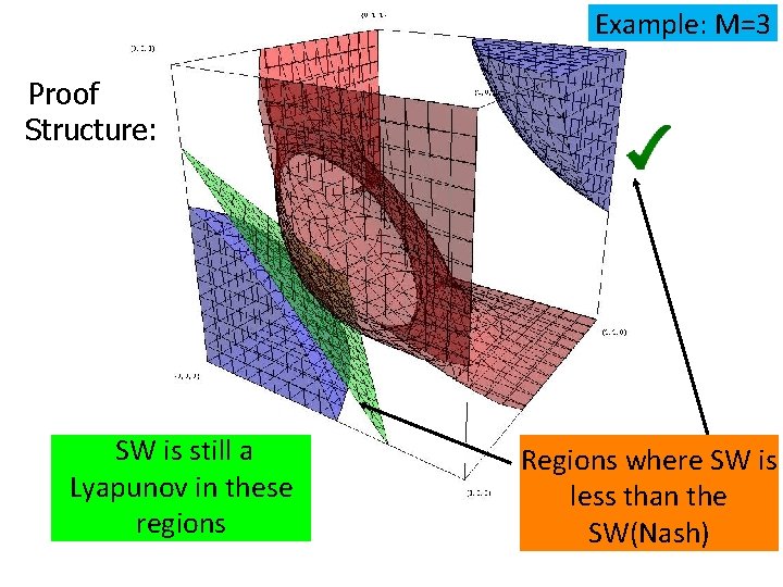
Example: M=3

Example: M=3 Proof Structure: SW is still a Lyapunov in these regions Regions where SW is less than the SW(Nash)

Example: M=3 Proof Structure: SW is still a Lyapunov in these regions Regions where SW is less than the SW(Nash)

Starting off the diagonal, we always escape these regions and we get trapped in the area with SW>SW(Nash)

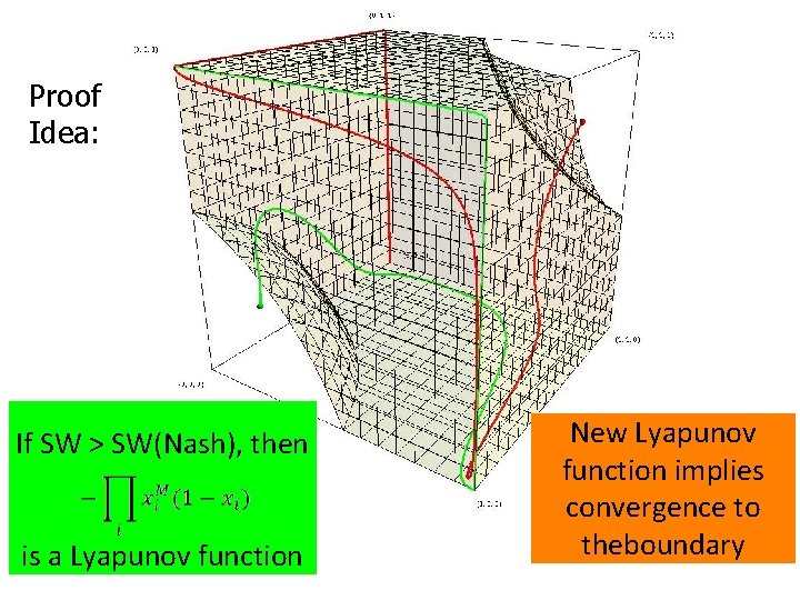
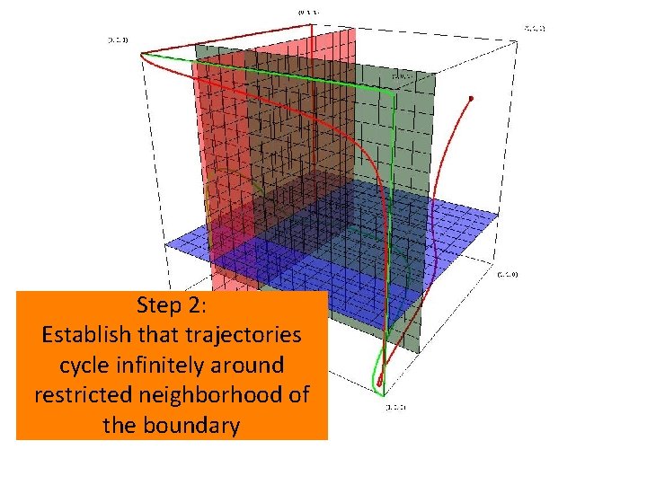
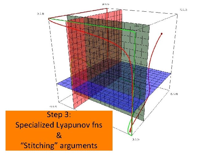
Proof Idea: If SW > SW(Nash), then is a Lyapunov function New Lyapunov function implies convergence to theboundary

Step 2: Establish that trajectories cycle infinitely Step 1: around Partition the space into regions whereof the restricted neighborhood growth rates of all strategies have fixed the boundary signs.

Step 3: Specialized Lyapunov fns & “Stitching” arguments

The Game* is ON *by game I mean projects