Introduction to Algorithms Spanning Trees CSE 680 Prof

Introduction to Algorithms Spanning Trees CSE 680 Prof. Roger Crawfis

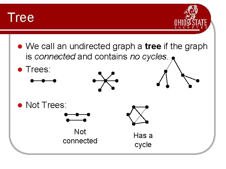
Tree We call an undirected graph a tree if the graph is connected and contains no cycles. l Trees: l l Not Trees: Not connected Has a cycle

Number of Vertices l If a graph is a tree, then the number of edges in the graph is one less than the number of vertices. l. A l tree with n vertices has n – 1 edges. Each node has one parent except for the root. l Note: Any node can be the root here, as we are not dealing with rooted trees.

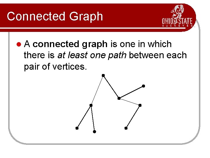
Connected Graph l. A connected graph is one in which there is at least one path between each pair of vertices.

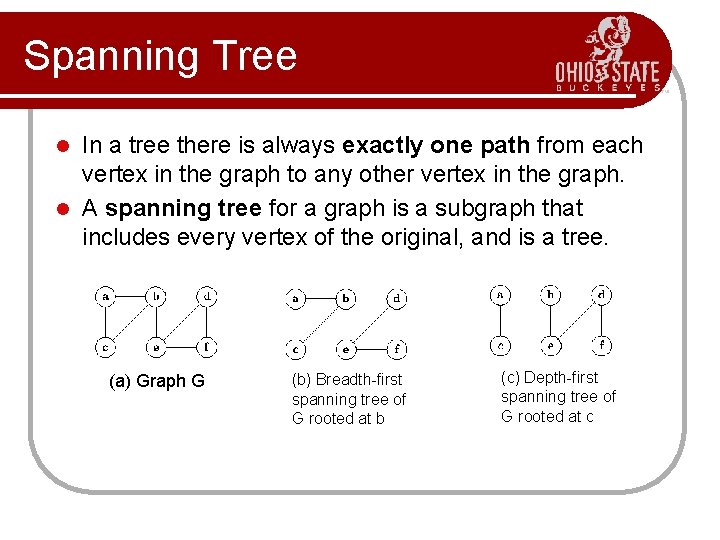
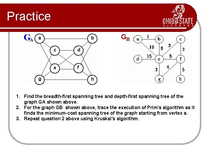
Spanning Tree In a tree there is always exactly one path from each vertex in the graph to any other vertex in the graph. l A spanning tree for a graph is a subgraph that includes every vertex of the original, and is a tree. l (a) Graph G (b) Breadth-first spanning tree of G rooted at b (c) Depth-first spanning tree of G rooted at c

Non-Connected Graphs l If the graph is not connected, we get a spanning tree for each connected component of the graph. l That is we get a forest.

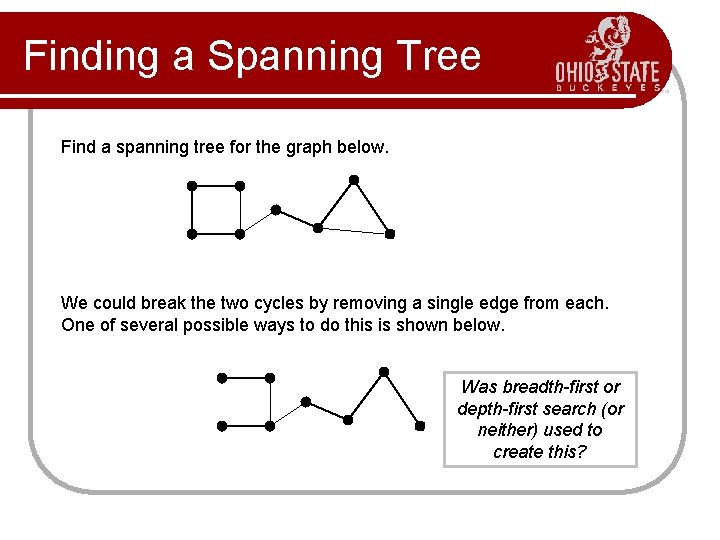
Finding a Spanning Tree Find a spanning tree for the graph below. We could break the two cycles by removing a single edge from each. One of several possible ways to do this is shown below. Was breadth-first or depth-first search (or neither) used to create this?

Minimum Spanning Tree l A spanning tree that has minimum total weight is called a minimum spanning tree for the graph. l l Technically it is a minimum-weight spanning tree. If all edges have the same weight, breadth-first search or depth-first search will yield minimum spanning trees. l For the rest of this discussion, we assume the edges have weights associated with them. Note, we are strictly dealing with undirected graphs here, for directed graphs we would want to find the optimum branching or aborescence of the directed graph.

Minimum Spanning Tree l Minimum-cost spanning trees have many applications. l l Building cable networks that join n locations with minimum cost. Building a road network that joins n cities with minimum cost. Obtaining an independent set of circuit equations for an electrical network. In pattern recognition minimal spanning trees can be used to find noisy pixels.

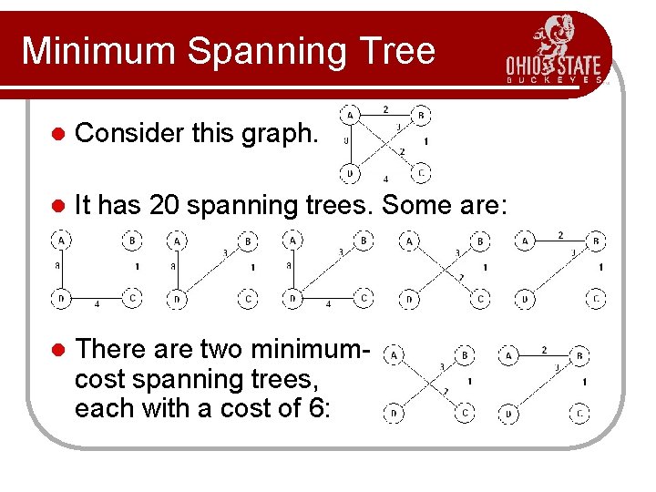
Minimum Spanning Tree l Consider this graph. l It has 20 spanning trees. Some are: l There are two minimumcost spanning trees, each with a cost of 6:

Minimum Spanning Tree l Brute Force option: For all possible spanning trees 1. i. ii. Calculate the sum of the edge weights Keep track of the tree with the minimum weight. Step i) requires N-1 time, since each tree will have exactly N-1 edges. l If there are M spanning trees, then the total cost will O(MN). l Consider a complete graph, with N(N-1) edges. How big can M be? l

Brute Force MST l For a complete graph, it has been shown that there are NN-2 possible spanning trees! l Alternatively, given N items, you can build NN-2 distinct trees to connect these items. l Note, for a lattice (like your grid implementation), the number of spanning trees is O(e 1. 167 N).

Minimum Spanning Tree There are many approaches to computing a minimum spanning tree. We could try to detect cycles and remove edges, but the two algorithms we will study build them from the bottom-up in a greedy fashion. l Kruskal’s Algorithm – starts with a forest of single node trees and then adds the edge with the minimum weight to connect two components. l Prim’s Algorithm – starts with a single vertex and then adds the minimum edge to extend the spanning tree. l

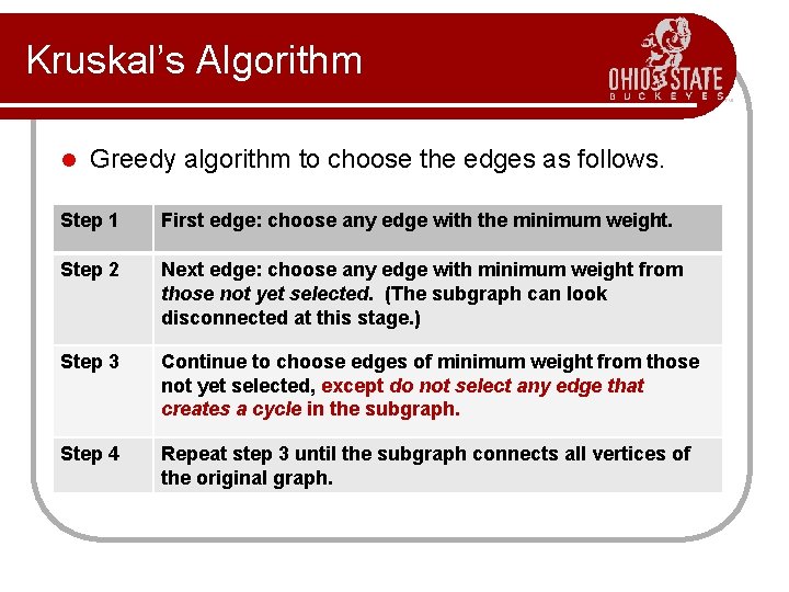
Kruskal’s Algorithm l Greedy algorithm to choose the edges as follows. Step 1 First edge: choose any edge with the minimum weight. Step 2 Next edge: choose any edge with minimum weight from those not yet selected. (The subgraph can look disconnected at this stage. ) Step 3 Continue to choose edges of minimum weight from those not yet selected, except do not select any edge that creates a cycle in the subgraph. Step 4 Repeat step 3 until the subgraph connects all vertices of the original graph.

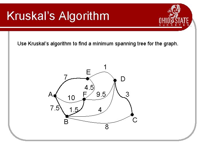
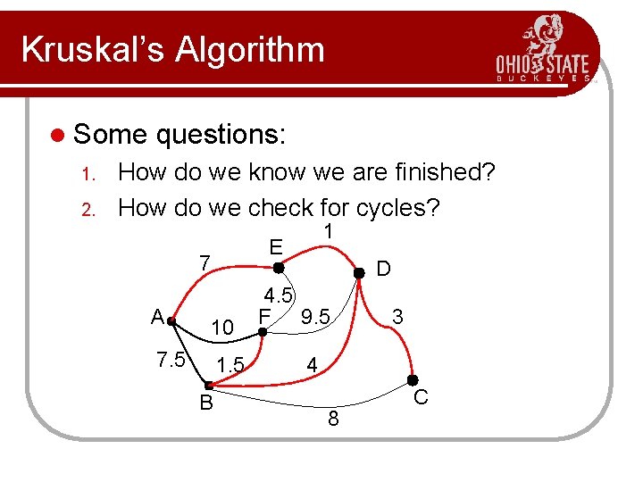
Kruskal’s Algorithm Use Kruskal’s algorithm to find a minimum spanning tree for the graph. E 7 A 10 7. 5 1. 5 B 1 D 4. 5 F 9. 5 3 4 8 C

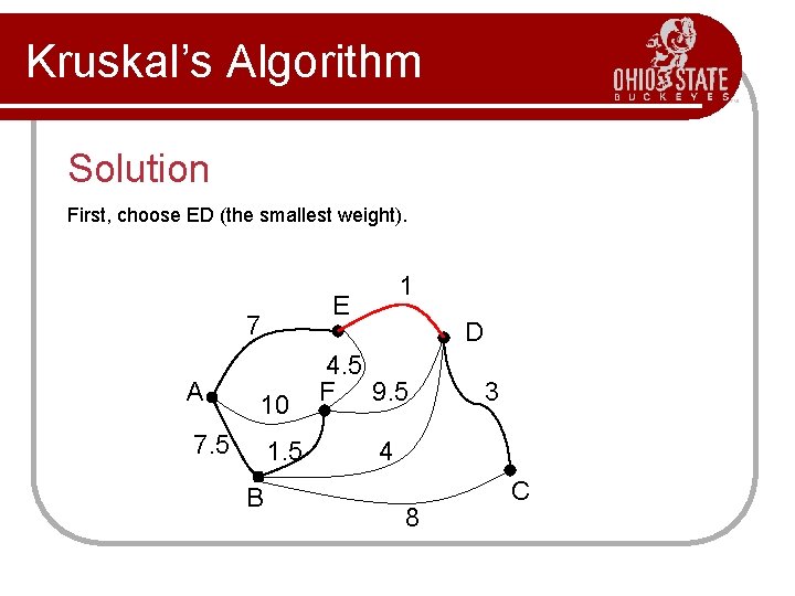
Kruskal’s Algorithm Solution First, choose ED (the smallest weight). E 7 A 10 7. 5 1. 5 B 1 D 4. 5 F 9. 5 3 4 8 C

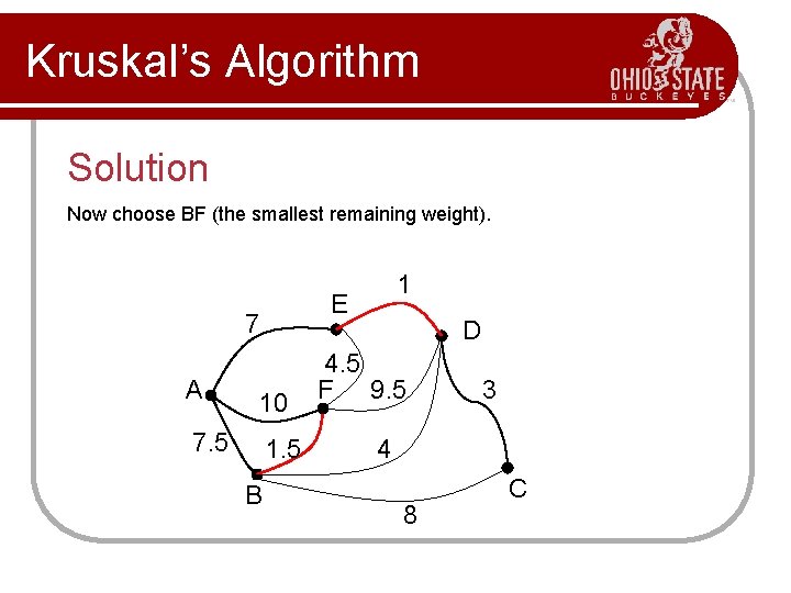
Kruskal’s Algorithm Solution Now choose BF (the smallest remaining weight). E 7 A 10 7. 5 1. 5 B 1 D 4. 5 F 9. 5 3 4 8 C

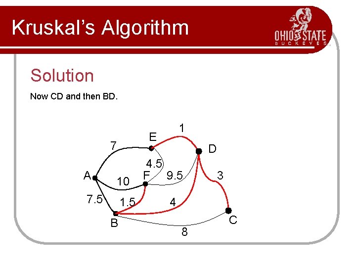
Kruskal’s Algorithm Solution Now CD and then BD. E 7 A 10 7. 5 1. 5 B 1 D 4. 5 F 9. 5 3 4 8 C

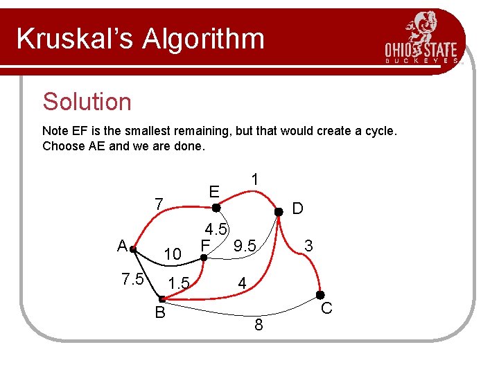
Kruskal’s Algorithm Solution Note EF is the smallest remaining, but that would create a cycle. Choose AE and we are done. E 7 A 10 7. 5 1. 5 B 1 D 4. 5 F 9. 5 3 4 8 C

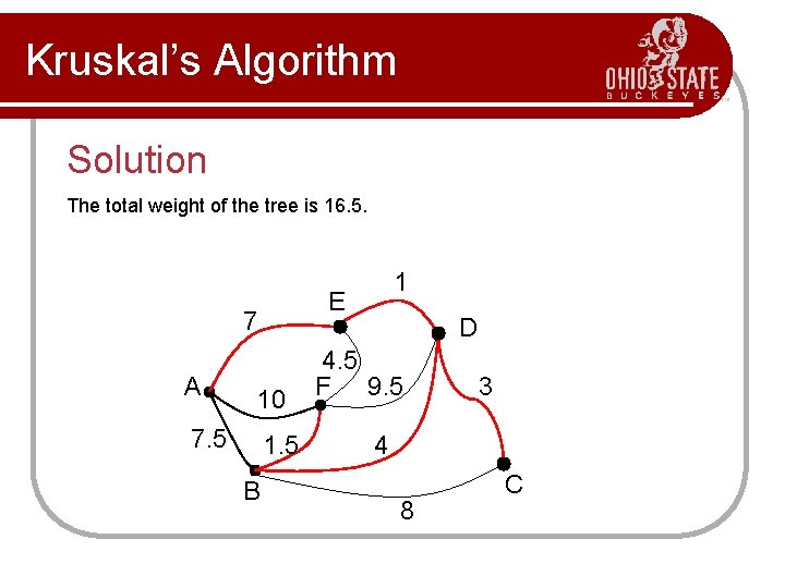
Kruskal’s Algorithm Solution The total weight of the tree is 16. 5. E 7 A 10 7. 5 1. 5 B 1 D 4. 5 F 9. 5 3 4 8 C

Kruskal’s Algorithm l Some 1. 2. questions: How do we know we are finished? How do we check for cycles? E 7 A 10 7. 5 1. 5 B 1 D 4. 5 F 9. 5 3 4 8 C

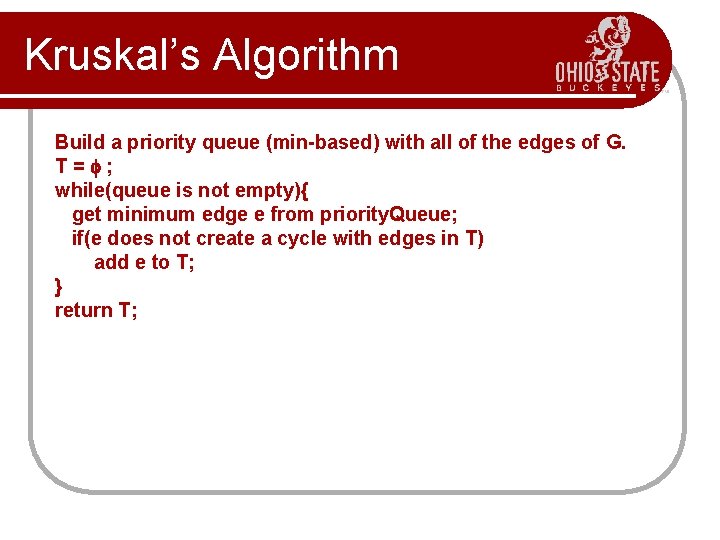
Kruskal’s Algorithm Build a priority queue (min-based) with all of the edges of G. T= ; while(queue is not empty){ get minimum edge e from priority. Queue; if(e does not create a cycle with edges in T) add e to T; } return T;

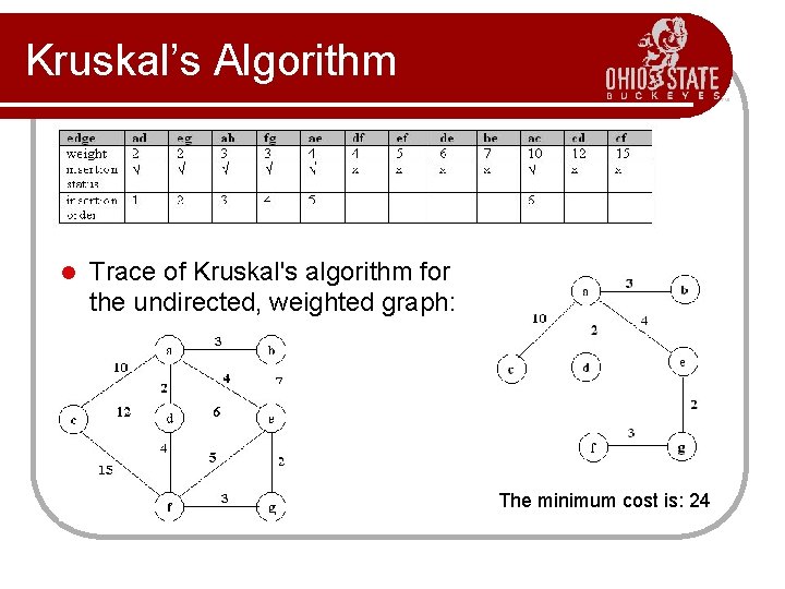
Kruskal’s Algorithm l Trace of Kruskal's algorithm for the undirected, weighted graph: The minimum cost is: 24

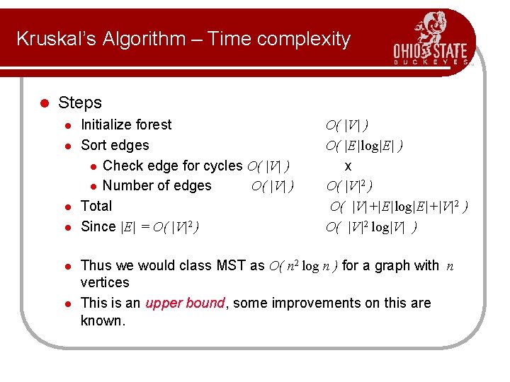
Kruskal’s Algorithm – Time complexity l Steps l l l Initialize forest Sort edges l Check edge for cycles O( |V| ) l Number of edges O( |V| ) Total Since |E| = O( |V|2 ) O( |V| ) O( |E|log|E| ) x O( |V|2 ) O( |V|+|E|log|E|+|V|2 ) O( |V|2 log|V| ) Thus we would class MST as O( n 2 log n ) for a graph with n vertices This is an upper bound, some improvements on this are known.

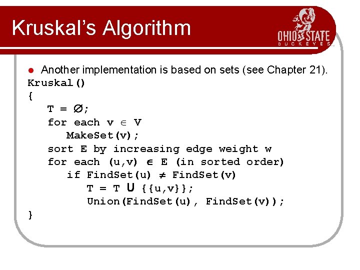
Kruskal’s Algorithm Another implementation is based on sets (see Chapter 21). Kruskal() { T = ; for each v V Make. Set(v); sort E by increasing edge weight w for each (u, v) E (in sorted order) if Find. Set(u) Find. Set(v) T = T U {{u, v}}; Union(Find. Set(u), Find. Set(v)); } l

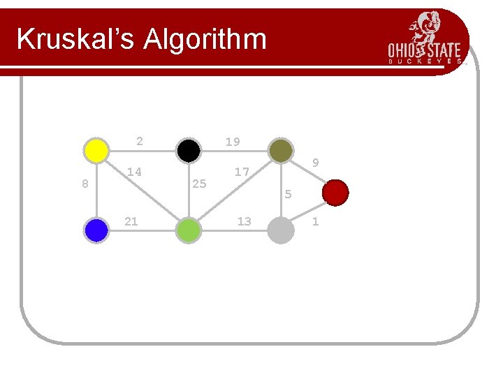
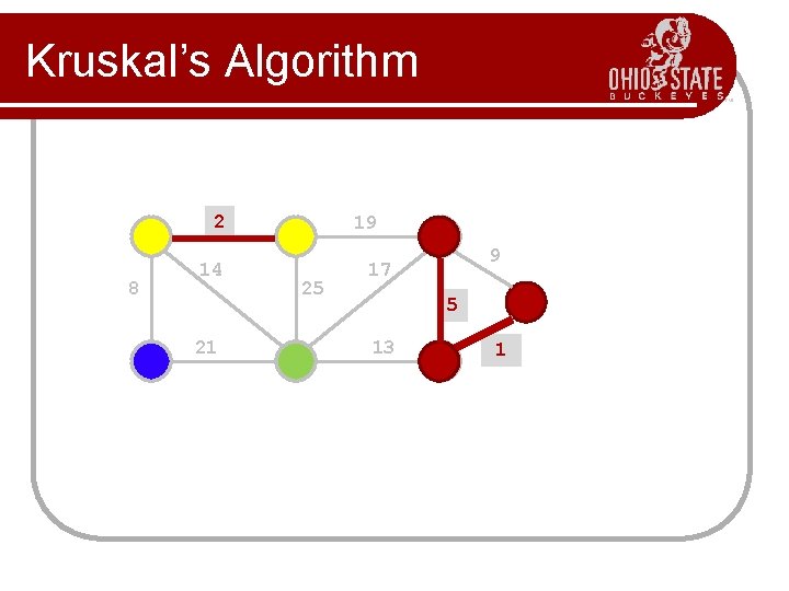
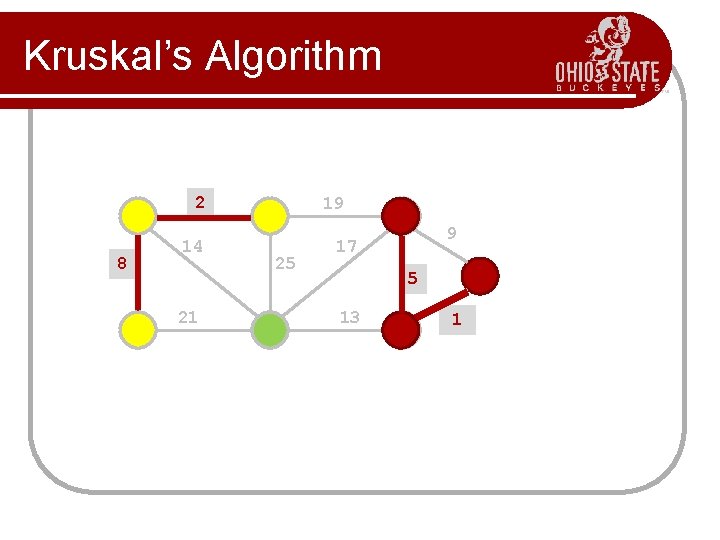
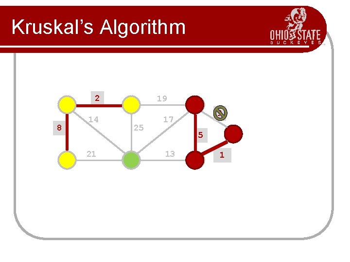
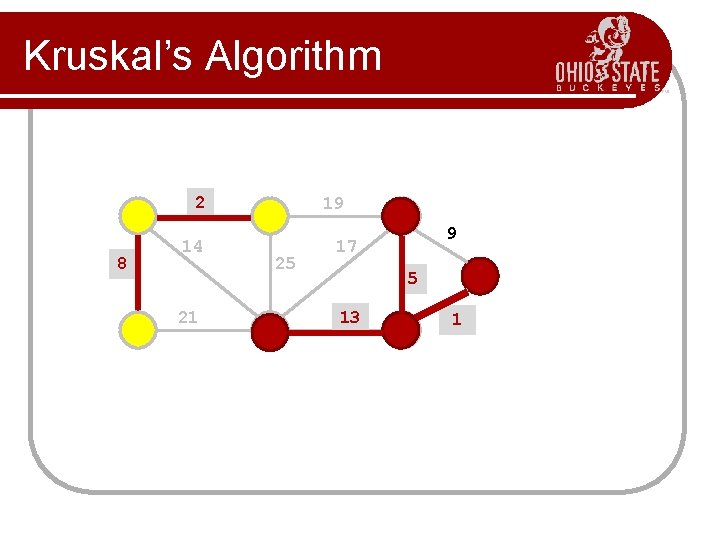
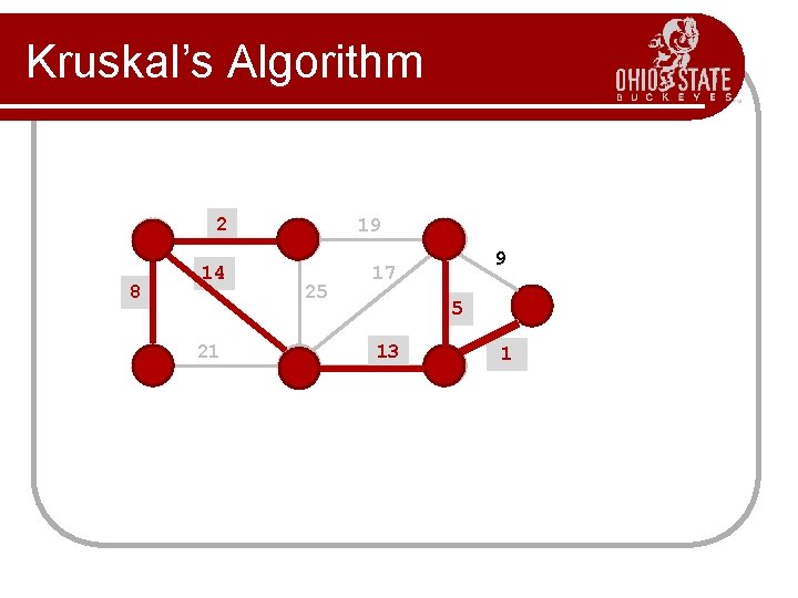
Kruskal’s Algorithm 2 8 14 21 19 25 9 17 5 13 1

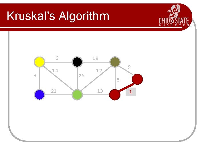
Kruskal’s Algorithm 2 8 14 21 19 25 9 17 5 13 1? 1

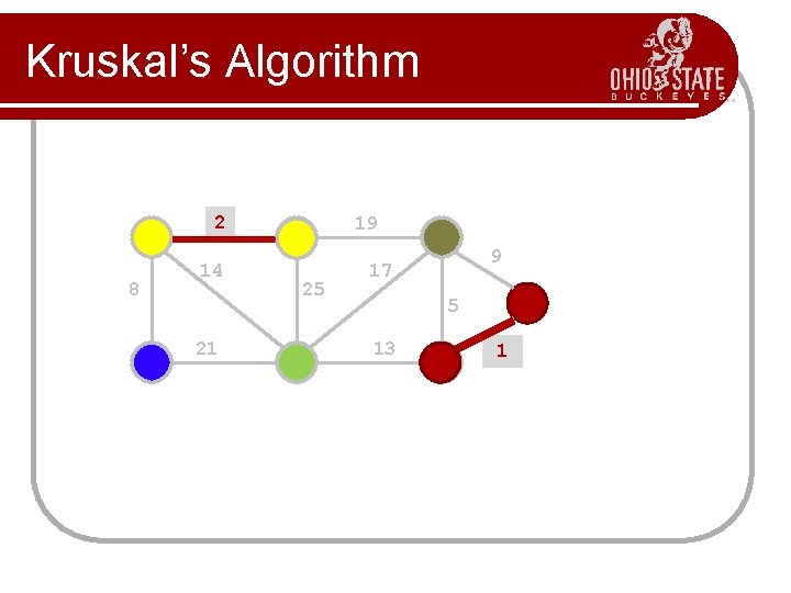
Kruskal’s Algorithm 2 8 14 21 19 25 9 17 5 13 1? 1

Kruskal’s Algorithm 2 8 14 21 19 25 9 17 5 13 1? 1

Kruskal’s Algorithm 2 8 14 21 19 25 9 17 5 13 1? 1

Kruskal’s Algorithm 2 8 14 21 19 25 9 17 5 13 1? 1

Kruskal’s Algorithm 2 8 14 21 19 25 9 17 5 13 1? 1

Kruskal’s Algorithm 2 8 14 21 19 25 9 17 5 13 1? 1

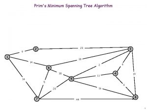
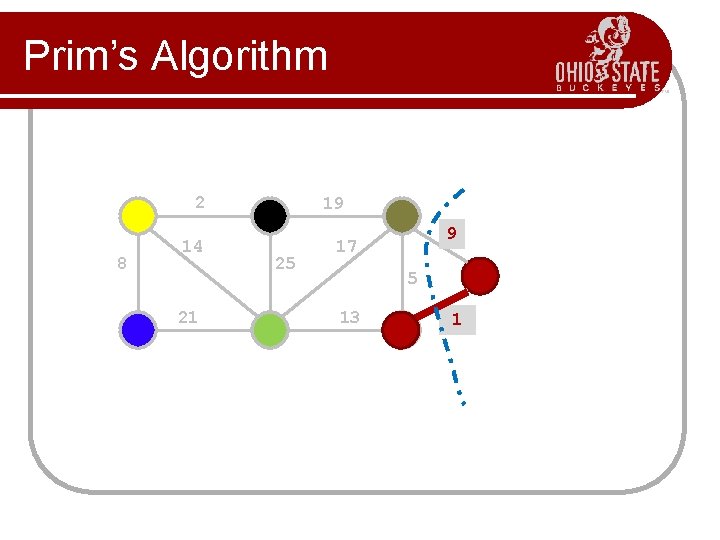
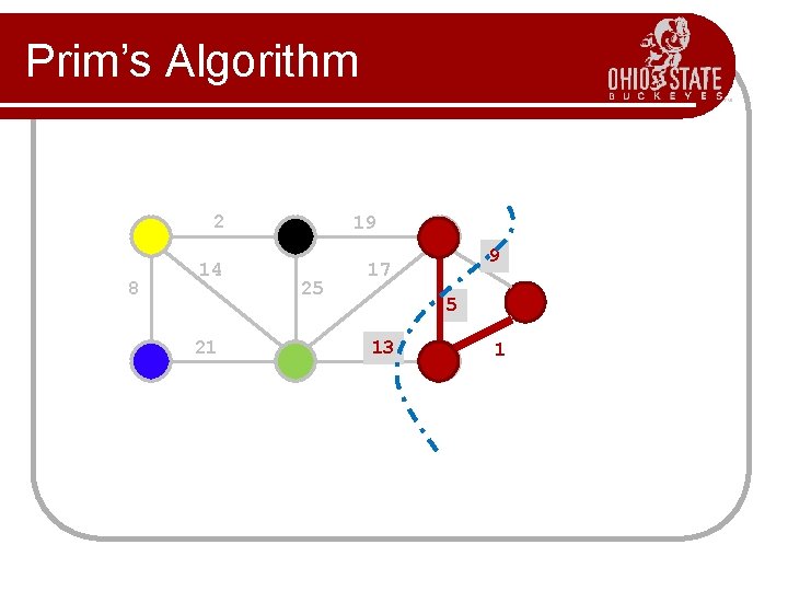
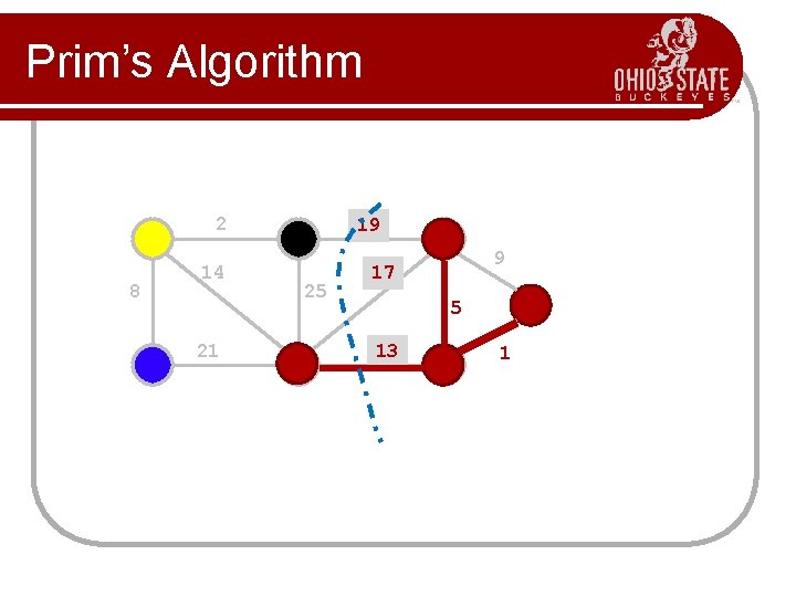
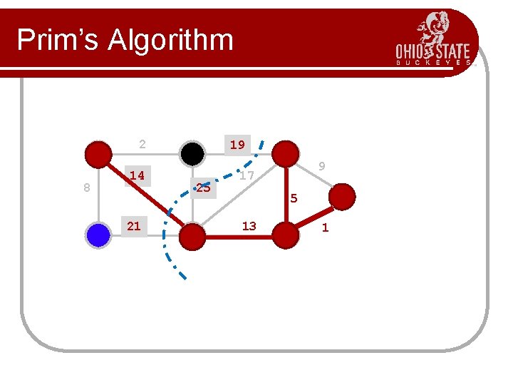
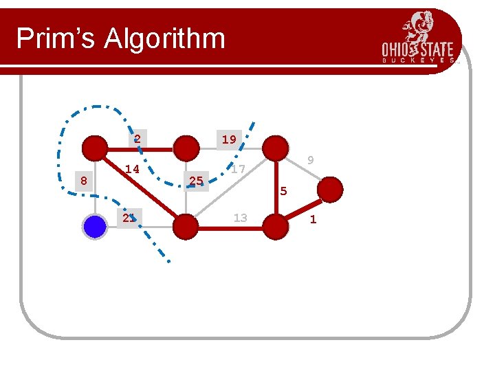
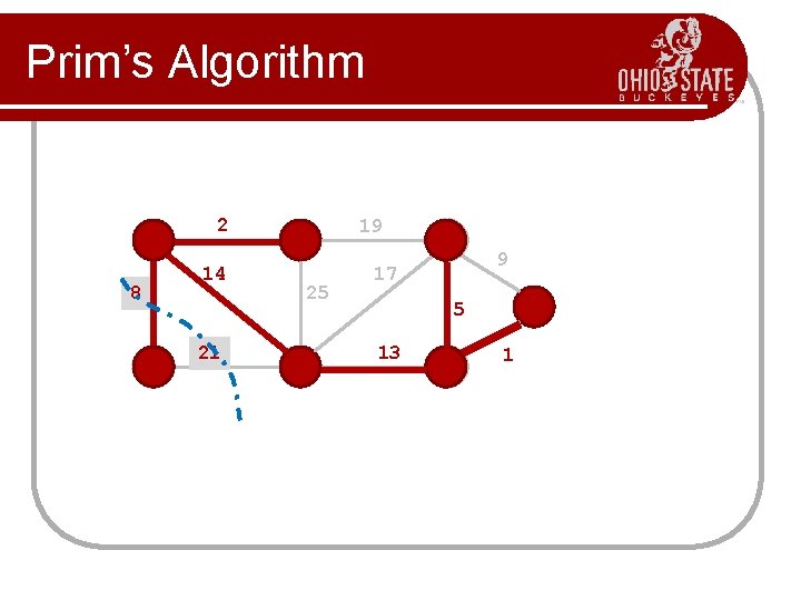
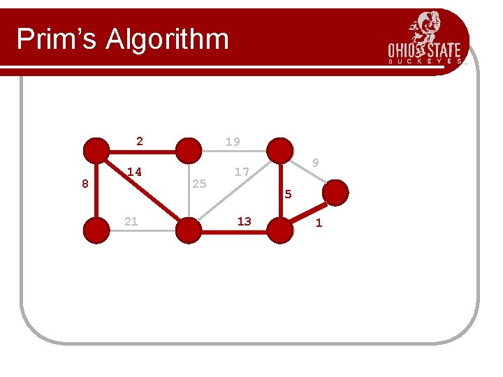
Prim’s Algorithm l l l Prim’s algorithm finds a minimum cost spanning tree by selecting edges from the graph one-by-one as follows: It starts with a tree, T, consisting of a single starting vertex, x. Then, it finds the shortest edge emanating from x that connects T to the rest of the graph (i. e. , a vertex not in the tree T). It adds this edge and the new vertex to the tree T. It then picks the shortest edge emanating from the revised tree T that also connects T to the rest of the graph and repeats the process.

Prim’s Algorithm Abstract Consider a graph G=(V, E); Let T be a tree consisting of only the starting vertex x; while (T has fewer than I V I vertices) { find a smallest edge connecting T to G-T; add it to T; }

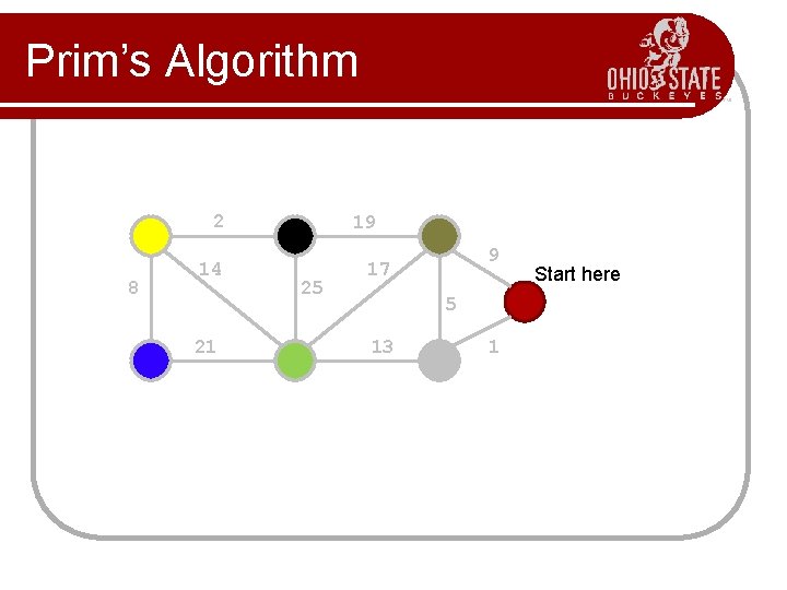
Prim’s Algorithm 2 8 14 21 19 25 9 17 5 13 1 Start here

Prim’s Algorithm 2 8 14 21 19 25 9 17 5 13 1? 1

Prim’s Algorithm 2 8 14 21 19 25 9 17 5 13 1

Prim’s Algorithm 2 8 14 21 19 25 9 17 5 13 1

Prim’s Algorithm 2 8 14 21 19 25 9 17 5 13 1

Prim’s Algorithm 2 8 14 21 19 25 9 17 5 13 1

Prim’s Algorithm 2 8 14 21 19 25 9 17 5 13 1

Prim’s Algorithm 2 8 14 21 19 25 9 17 5 13 1

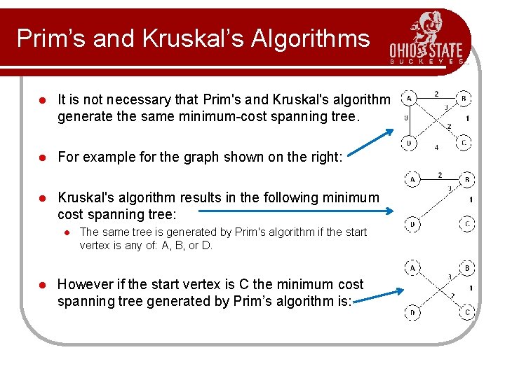
Prim’s and Kruskal’s Algorithms l It is not necessary that Prim's and Kruskal's algorithm generate the same minimum-cost spanning tree. l For example for the graph shown on the right: l Kruskal's algorithm results in the following minimum cost spanning tree: l l The same tree is generated by Prim's algorithm if the start vertex is any of: A, B, or D. However if the start vertex is C the minimum cost spanning tree generated by Prim’s algorithm is:

Implementation Details Prim’s Algorithm from your book is horrible from a SE stand-point! MST-Prim(G, w, r) Q is a priority queue Q = V[G]; key is the internal priorities in Q! for each u Q changing key, changes the queue. key[u] = ; key[r] = 0; p[r] = NULL; while (Q not empty) u = Extract. Min(Q); for each v Adj[u] if (v Q and w(u, v) < key[v]) p[v] = u; key[v] = w(u, v); l

Implementation Details Why queue the vertices, rather than the newly discovered edges? MST-Prim(G, w, r) Q = V[G]; A Fibonacci Heap allows this to be for each u Q done in O(1) time. key[u] = ; l Decrease. Key(r, 0); p[r] = NULL; while (Q not empty) u = Extract. Min(Q); for each v Adj[u] if (v Q and w(u, v) < key[v]) p[v] = u; Decrease. Key(v, w(u, v));

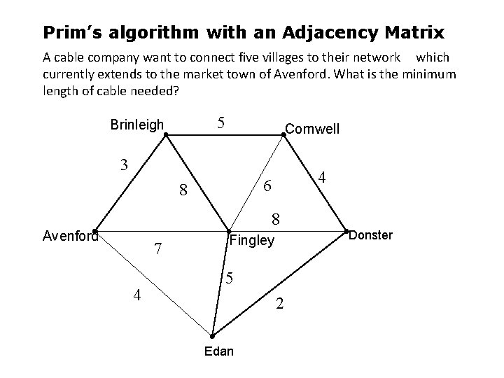
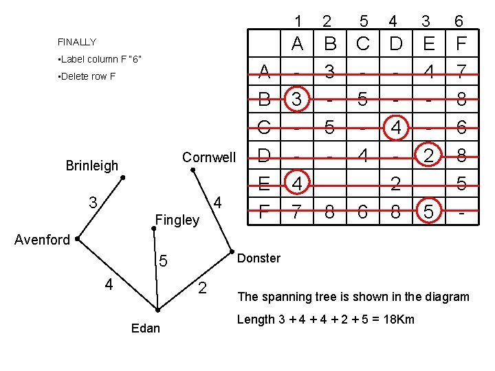
Prim’s algorithm with an Adjacency Matrix A cable company want to connect five villages to their network which currently extends to the market town of Avenford. What is the minimum length of cable needed? 5 Brinleigh Cornwell 3 4 6 8 8 Avenford 7 4 Fingley 5 2 Edan Donster

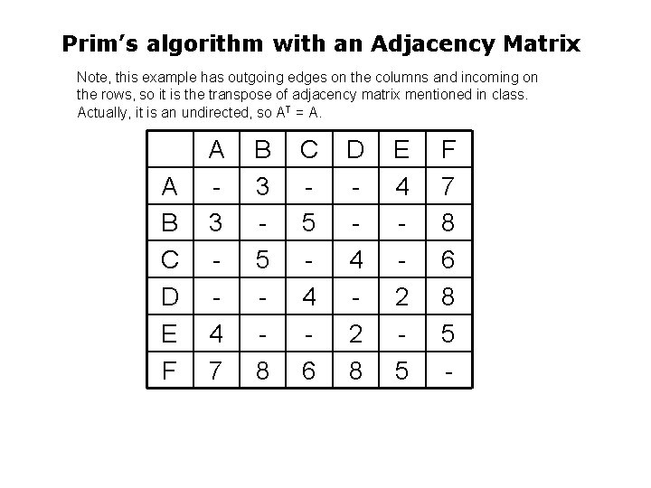
Prim’s algorithm with an Adjacency Matrix Note, this example has outgoing edges on the columns and incoming on the rows, so it is the transpose of adjacency matrix mentioned in class. Actually, it is an undirected, so AT = A. A B C D E F A 3 4 7 B 3 5 8 C 5 4 6 D 4 2 8 E 4 2 5 F 7 8 6 8 5 -

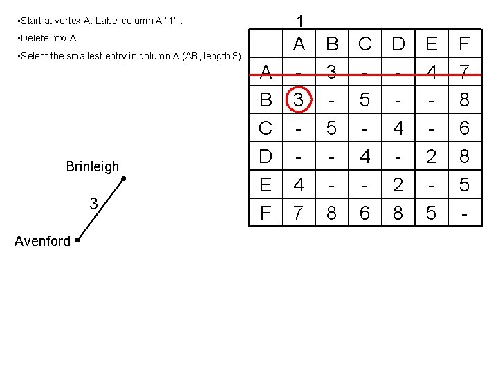
1 • Start at vertex A. Label column A “ 1”. • Delete row A • Select the smallest entry in column A (AB, length 3) Brinleigh 3 Avenford A B C D E F A 3 4 7 B 3 5 8 C D - 5 - 4 4 - 2 6 8 E 4 2 5 F 7 8 6 8 5 -

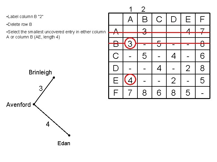
• Label column B “ 2” • Delete row B • Select the smallest uncovered entry in either column A or column B (AE, length 4) Brinleigh 3 Avenford 4 Edan A B C D E F 1 2 A 3 4 7 B 3 5 8 C D - 5 - 4 4 - 2 6 8 E 4 2 5 F 7 8 6 8 5 -

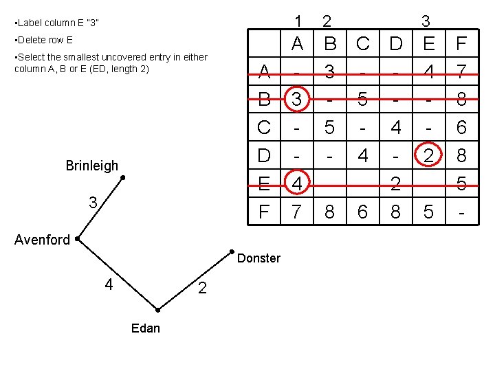
• Label column E “ 3” • Delete row E • Select the smallest uncovered entry in either column A, B or E (ED, length 2) Brinleigh 3 A B C D E F Avenford Donster 4 2 Edan 1 2 A 3 4 7 B 3 5 8 3 C D - 5 - 4 4 - 2 6 8 E 4 2 5 F 7 8 6 8 5 -

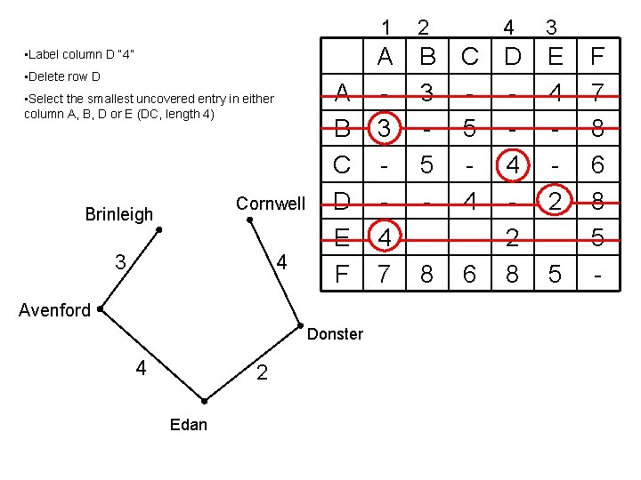
• Label column D “ 4” • Delete row D • Select the smallest uncovered entry in either column A, B, D or E (DC, length 4) Cornwell Brinleigh 4 3 A B C D E F Avenford Donster 4 2 Edan 1 2 A 3 4 7 B 3 5 8 4 C D - 5 - 4 4 - 2 6 8 3 E 4 2 5 F 7 8 6 8 5 -

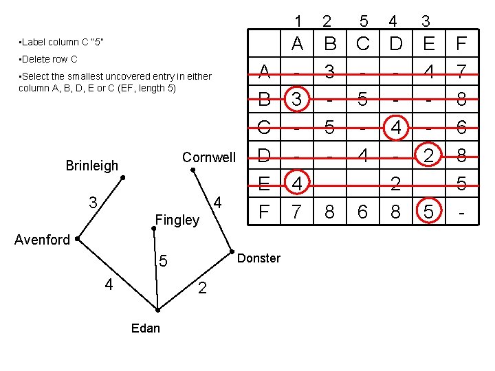
• Label column C “ 5” • Delete row C • Select the smallest uncovered entry in either column A, B, D, E or C (EF, length 5) Cornwell Brinleigh 4 3 Fingley A B C D E F Avenford Donster 5 4 2 Edan 1 2 5 4 A 3 4 7 B 3 5 8 C D - 5 - 4 4 - 2 6 8 3 E 4 2 5 F 7 8 6 8 5 -

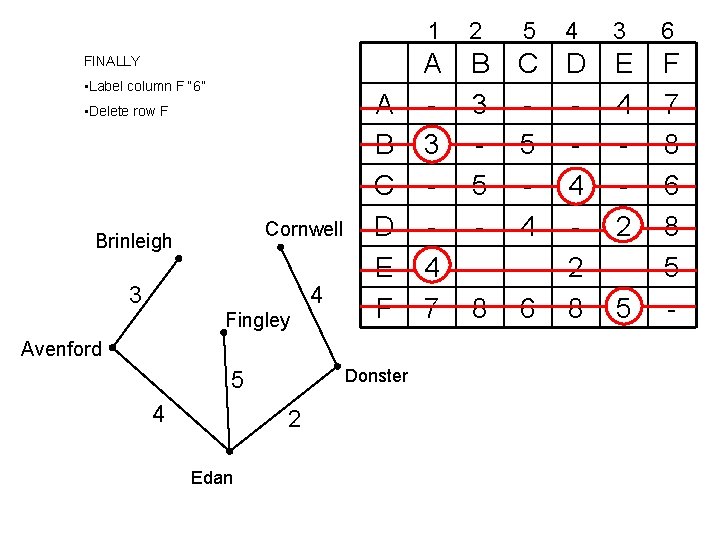
FINALLY • Label column F “ 6” • Delete row F Cornwell Brinleigh 4 3 Fingley A B C D E F Avenford Donster 5 4 2 Edan 1 2 5 4 A 3 4 7 B 3 5 8 C D - 5 - 4 4 - 2 6 8 3 6 E 4 2 5 F 7 8 6 8 5 -

FINALLY • Label column F “ 6” • Delete row F Cornwell Brinleigh 4 3 Fingley A B C D E F 1 2 5 4 A 3 4 7 B 3 5 8 C D - 5 - 4 4 - 2 6 8 3 6 E 4 2 5 F 7 8 6 8 5 - Avenford Donster 5 4 2 Edan The spanning tree is shown in the diagram Length 3 + 4 + 2 + 5 = 18 Km

Practice GB 1. Find the breadth-first spanning tree and depth-first spanning tree of the graph GA shown above. 2. For the graph GB shown above, trace the execution of Prim's algorithm as it finds the minimum-cost spanning tree of the graph starting from vertex a. 3. Repeat question 2 above using Kruskal's algorithm.

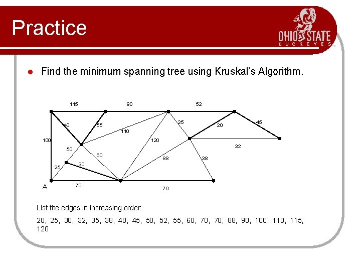
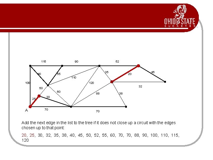
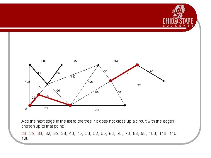
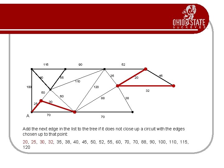
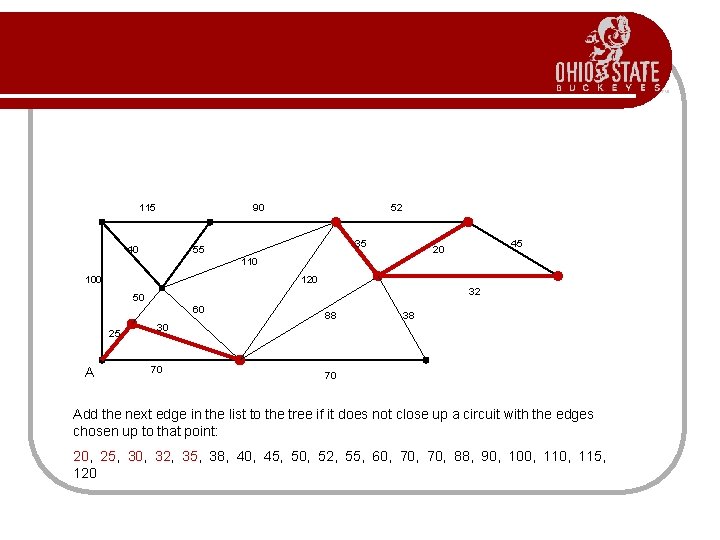
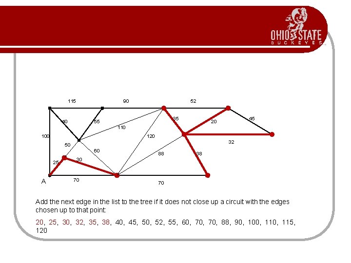
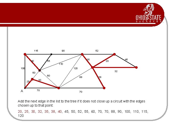
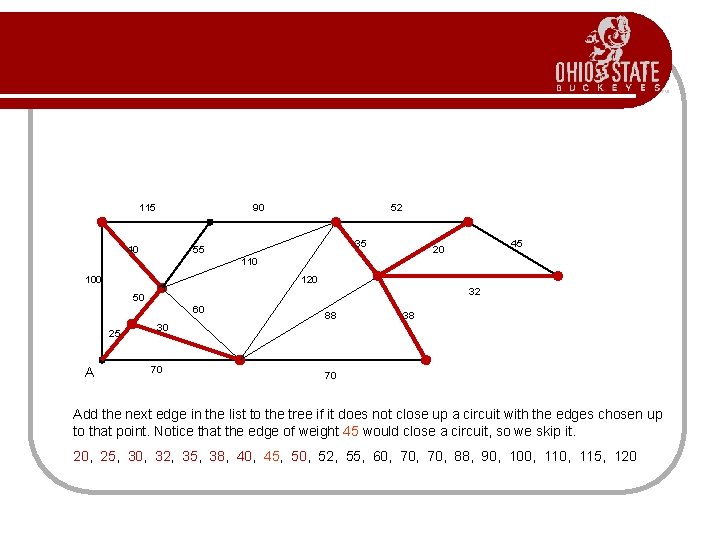
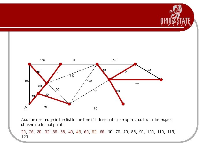
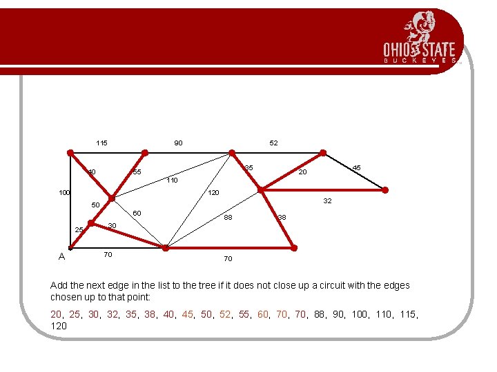
Practice l Find the minimum spanning tree using Kruskal’s Algorithm. 115 90 40 52 35 55 45 20 110 100 120 32 50 60 25 A 88 38 30 70 70 List the edges in increasing order: 20, 25, 30, 32, 35, 38, 40, 45, 50, 52, 55, 60, 70, 88, 90, 100, 115, 120

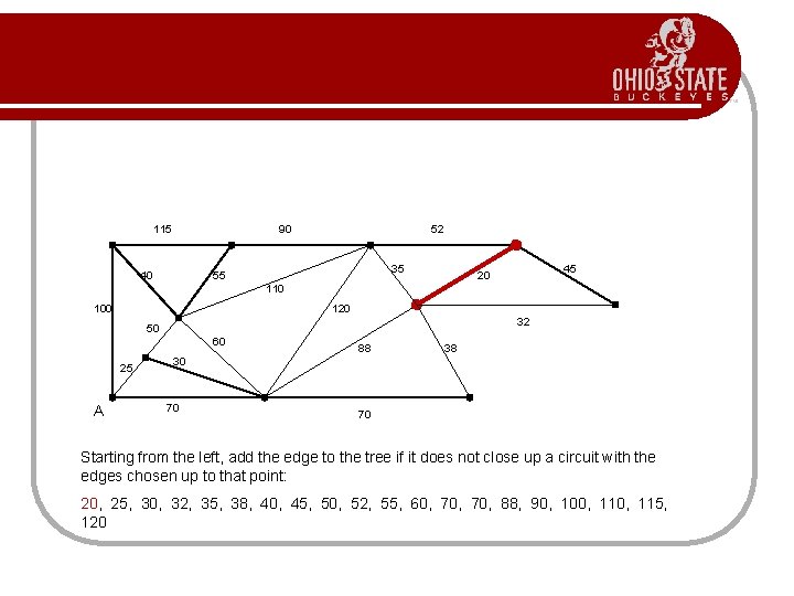
115 90 40 52 35 55 45 20 110 100 120 32 50 60 25 A 88 38 30 70 70 Starting from the left, add the edge to the tree if it does not close up a circuit with the edges chosen up to that point: 20, 25, 30, 32, 35, 38, 40, 45, 50, 52, 55, 60, 70, 88, 90, 100, 115, 120

115 90 40 52 35 55 45 20 110 100 120 32 50 60 25 A 88 38 30 70 70 Add the next edge in the list to the tree if it does not close up a circuit with the edges chosen up to that point: 20, 25, 30, 32, 35, 38, 40, 45, 50, 52, 55, 60, 70, 88, 90, 100, 115, 120

115 90 40 52 35 55 45 20 110 100 120 32 50 60 25 A 88 38 30 70 70 Add the next edge in the list to the tree if it does not close up a circuit with the edges chosen up to that point: 20, 25, 30, 32, 35, 38, 40, 45, 50, 52, 55, 60, 70, 88, 90, 100, 115, 120

115 90 40 52 35 55 45 20 110 100 120 32 50 60 25 A 88 38 30 70 70 Add the next edge in the list to the tree if it does not close up a circuit with the edges chosen up to that point: 20, 25, 30, 32, 35, 38, 40, 45, 50, 52, 55, 60, 70, 88, 90, 100, 115, 120

115 90 40 52 35 55 45 20 110 100 120 32 50 60 25 A 88 38 30 70 70 Add the next edge in the list to the tree if it does not close up a circuit with the edges chosen up to that point: 20, 25, 30, 32, 35, 38, 40, 45, 50, 52, 55, 60, 70, 88, 90, 100, 115, 120

115 90 40 52 35 55 45 20 110 100 120 32 50 60 25 A 88 38 30 70 70 Add the next edge in the list to the tree if it does not close up a circuit with the edges chosen up to that point: 20, 25, 30, 32, 35, 38, 40, 45, 50, 52, 55, 60, 70, 88, 90, 100, 115, 120

115 90 40 52 35 55 45 20 110 100 120 32 50 60 25 A 88 38 30 70 70 Add the next edge in the list to the tree if it does not close up a circuit with the edges chosen up to that point: 20, 25, 30, 32, 35, 38, 40, 45, 50, 52, 55, 60, 70, 88, 90, 100, 115, 120

115 90 40 52 35 55 45 20 110 100 120 32 50 60 25 A 88 38 30 70 70 Add the next edge in the list to the tree if it does not close up a circuit with the edges chosen up to that point. Notice that the edge of weight 45 would close a circuit, so we skip it. 20, 25, 30, 32, 35, 38, 40, 45, 50, 52, 55, 60, 70, 88, 90, 100, 115, 120

115 90 40 52 35 55 45 20 110 100 120 32 50 60 25 A 88 38 30 70 70 Add the next edge in the list to the tree if it does not close up a circuit with the edges chosen up to that point: 20, 25, 30, 32, 35, 38, 40, 45, 50, 52, 55, 60, 70, 88, 90, 100, 115, 120

115 90 40 52 35 55 45 20 110 100 120 32 50 60 25 A 88 38 30 70 70 Add the next edge in the list to the tree if it does not close up a circuit with the edges chosen up to that point: 20, 25, 30, 32, 35, 38, 40, 45, 50, 52, 55, 60, 70, 88, 90, 100, 115, 120

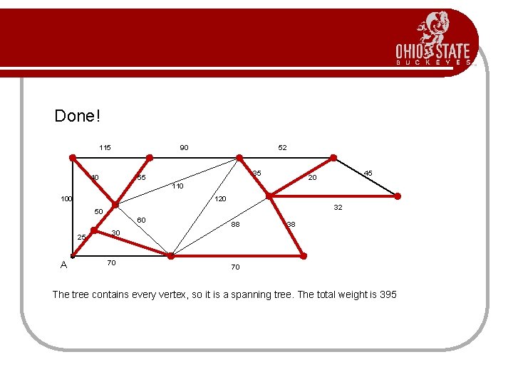
Done! 115 90 40 52 35 55 45 20 110 100 120 32 50 60 25 A 88 38 30 70 70 The tree contains every vertex, so it is a spanning tree. The total weight is 395

Kruskal vs. Prim l Both are Greedy algorithms l l l Different sets of edges considered l l Kruskal – set containment and union. Prim – Simple boolean. Both can terminate early l l l Kruskal – all edges Prim – Edges from Tree nodes to rest of G. Both need to check for cycles l l Both take the next minimum edge Both are optimal (find the global min) Kruskal – when |V|-1 edges are added. Prim – when |V| nodes are added (or |V|-1 edges). Both are O( |E| log|V| ) l l Prim can be O( |E| + |V| log|V| ) w/ Fibonacci Heaps Prim with an adjacency matrix is O(|V|2).