Introducing POW 1 22 How to get more

Introducing POW! 1. 22 How to get more out of your data - but not too much ! 1

Introducing POW! 1. 22 Programme for today § Overview and catch-up on the POW! Framework § Using maths to solve problems • Principal components, Robust components and Missing data • What do I do if my forecasts are partly based on history ? § Using algorithms to do the hard work • Compound linear constraints: protection against the unexpected • What if history had been different ? › The balanced, block and calendar bootstrap § Property is different: what can it teach us ? • Direct or indirect ? How can an investor decide ? › POW! applied to the IPD / OCCAM UK and Global property models • Probability-adjusted cash-flow modelling with PAC-M § Flash presentations 2

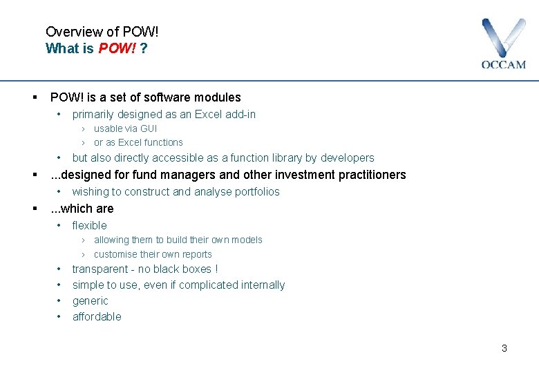
Overview of POW! What is POW! ? § POW! is a set of software modules • primarily designed as an Excel add-in › usable via GUI › or as Excel functions • § . . . designed for fund managers and other investment practitioners • § but also directly accessible as a function library by developers wishing to construct and analyse portfolios . . . which are • flexible › allowing them to build their own models › customise their own reports • • transparent - no black boxes ! simple to use, even if complicated internally generic affordable 3

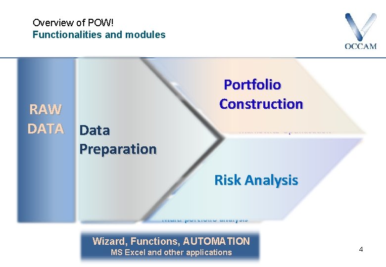
Overview of POW! Functionalities and modules BAYES Refine Risk/Return forecasts BACKTEST Multi-period backtest RAW TOOLBOX Calculate asset covariances DATA Data with optional: - observation weights Preparation - TS/PCA factors Fill missing data PROPERTY Model Real Estate Portfolio ROBUST Bootstrap Optimisation Construction FRONTIER Markowitz Optimisation RISK Risk/Return Analysis EMPIRICAL Risk Analysis Empirical & Simulations MANDATE Multi-portfolio analysis Wizard, Functions, AUTOMATION MS Excel and other applications 4

Overview of POW! Lightning demo ! 5

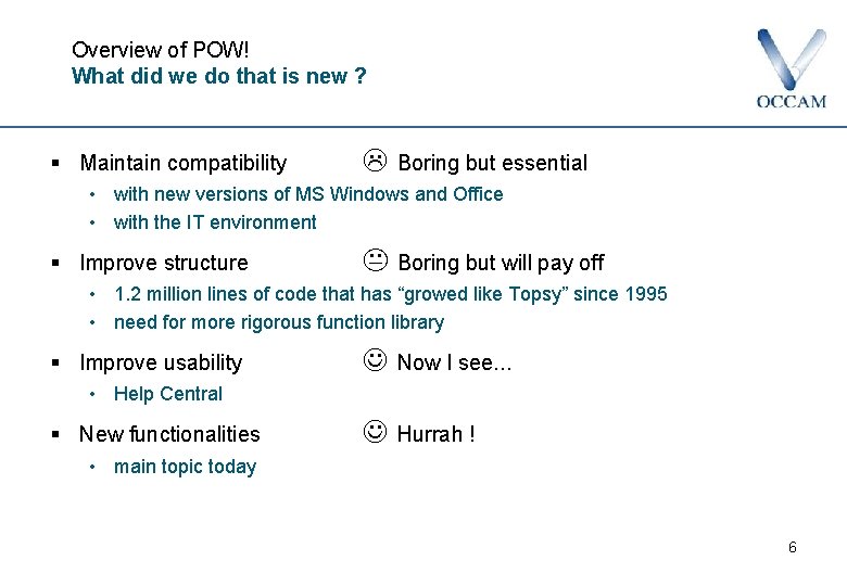
Overview of POW! What did we do that is new ? § Maintain compatibility Boring but essential • with new versions of MS Windows and Office • with the IT environment § Improve structure Boring but will pay off • 1. 2 million lines of code that has “growed like Topsy” since 1995 • need for more rigorous function library § Improve usability Now I see. . . • Help Central § New functionalities Hurrah ! • main topic today 6

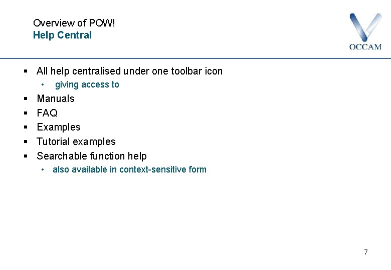
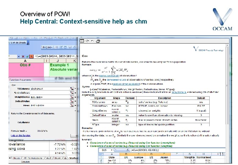
Overview of POW! Help Central § All help centralised under one toolbar icon • § § § giving access to Manuals FAQ Examples Tutorial examples Searchable function help • also available in context-sensitive form 7

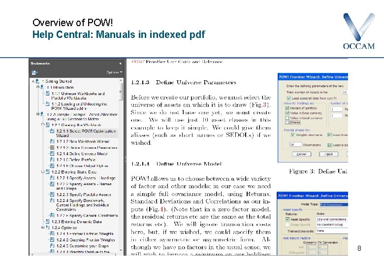
Overview of POW! Help Central: Manuals in indexed pdf 8

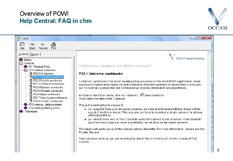
Overview of POW! Help Central: FAQ in chm 9

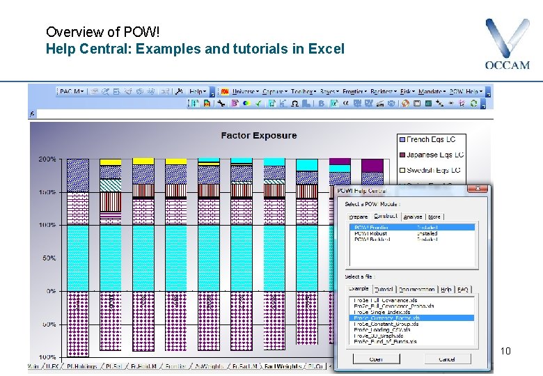
Overview of POW! Help Central: Examples and tutorials in Excel 10

Overview of POW! Help Central: Context-sensitive help as chm 11

Introducing POW! 1. 22 Principal Components Robust Components Missing data 12

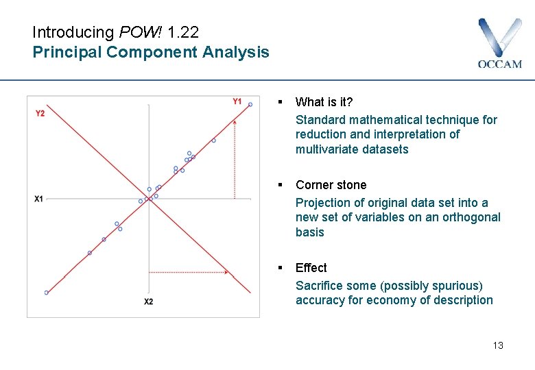
Introducing POW! 1. 22 Principal Component Analysis § What is it? Standard mathematical technique for reduction and interpretation of multivariate datasets § Corner stone Projection of original data set into a new set of variables on an orthogonal basis § Effect Sacrifice some (possibly spurious) accuracy for economy of description 13

Introducing POW! 1. 22 Principal Component Analysis § Benefits: • Capture the underlying trends by identifying parameter correlations • Data compression, which is important when analyzing large data sets • Used as inputs in statistical factor models • Useful when choice of fundamental or macro factors is unclear § Possible financial applications: • Portfolio construction Remove noise and control exposure to the main drivers of the market structure • Forecasting Anything that might be useful as an indicator of future events • Trading strategy Trend duration – PCA could shed some lights on Market Memory. 14

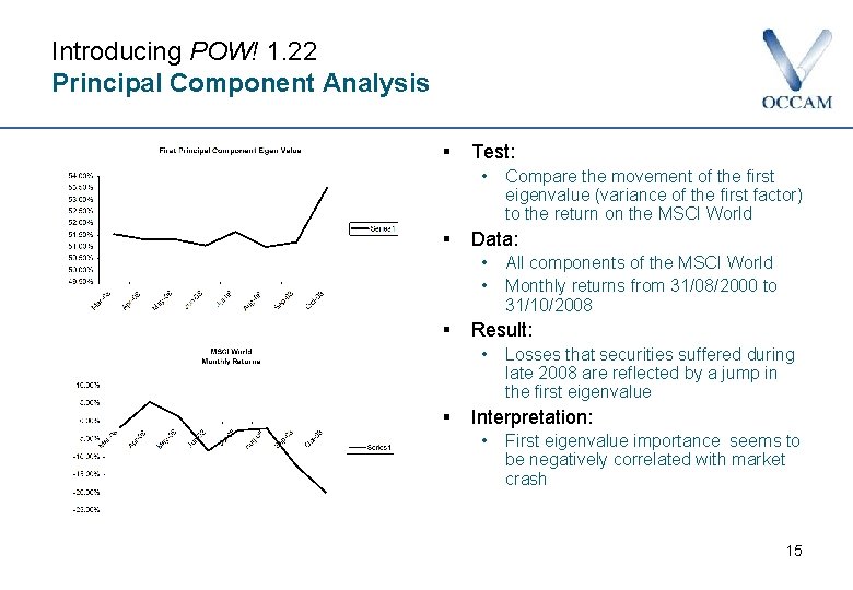
Introducing POW! 1. 22 Principal Component Analysis § Test: • § Data: • • § All components of the MSCI World Monthly returns from 31/08/2000 to 31/10/2008 Result: • § Compare the movement of the first eigenvalue (variance of the first factor) to the return on the MSCI World Losses that securities suffered during late 2008 are reflected by a jump in the first eigenvalue Interpretation: • First eigenvalue importance seems to be negatively correlated with market crash 15

Introducing POW! 1. 22 Robust Component Analysis § What is RCA ? An intuitive, iterative way to think about PCA • • § Same results as in PCA taking a different path Has all PCA’s bells and whistle functions and even more… How it works • • Imagine you built an index of (say) FT chemicals. . . then adjusted the index for the betas of the components. . . then calculated betas to the new index. . . then adjusted the index. . . › • • and so on until it converges You would have the first eigenvector. . then repeat for the unexplained residuals n time › and you would have a PCA model 16

Introducing POW! 1. 22 Robust Component Analysis § Strength is its flexibility • Can control betas (eg no beta <0 or >1) • Can divide time-series into logical groups › • eg regions within the MSCI World, but still allow some markets (eg US) to be shared by all groups) Can be used to fill and model gappy data › › some markets closed for public holiday data needed monthly but some only available quarterly short time series (eg recently launched funds) markets slow to release data (eg Japanese property) 17

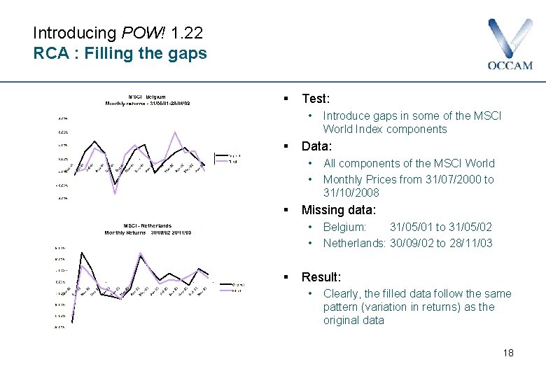
Introducing POW! 1. 22 RCA : Filling the gaps § Test: • § Data: • • § All components of the MSCI World Monthly Prices from 31/07/2000 to 31/10/2008 Missing data: • • § Introduce gaps in some of the MSCI World Index components Belgium: 31/05/01 to 31/05/02 Netherlands: 30/09/02 to 28/11/03 Result: • Clearly, the filled data follow the same pattern (variation in returns) as the original data 18

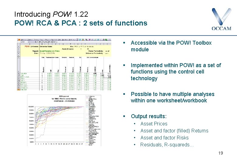
Introducing POW! 1. 22 POW! RCA & PCA : 2 sets of functions § Accessible via the POW! Toolbox module § Implemented within POW! as a set of functions using the control cell technology § Possible to have multiple analyses within one worksheet/workbook § Output results: • • Asset Prices Asset and factor (filled) Returns Asset and factor Risks Residuals, R-squareds. . . 19

Introducing POW! 1. 22 What do I do when my Forecasts are partly based on history? Correcting the hidden assumptions of Black-Litterman 20

What do I do when my Forecasts are partly based on history? Correcting the hidden assumptions of Black-Litterman § The problem to solve § The Bayesian forecasting procedure § The non-orthogonal Bayesian formalism § The Bayesian Black-Litterman (BL) model § Numerical exploration of non-orthogonal BL 21

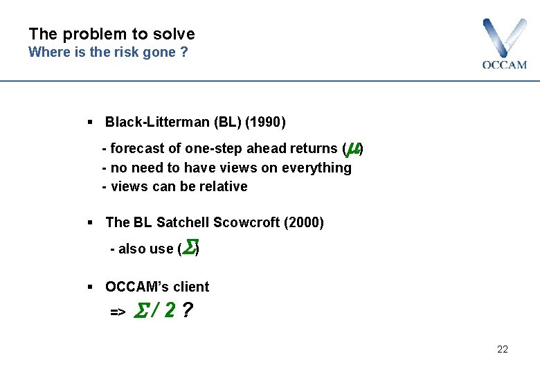
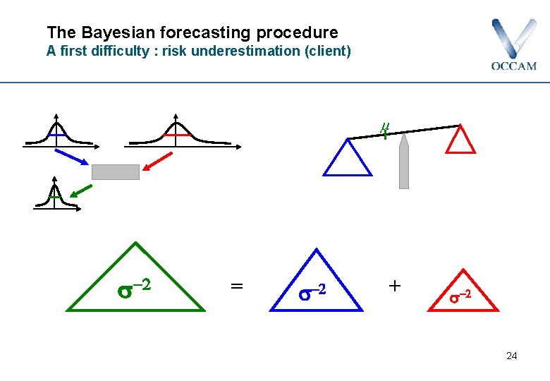
The problem to solve Where is the risk gone ? § Black-Litterman (BL) (1990) - forecast of one-step ahead returns ( ) - no need to have views on everything - views can be relative § The BL Satchell Scowcroft (2000) - also use ( ) § OCCAM’s client => /2? 22

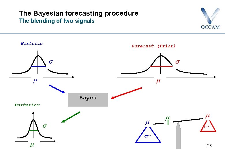
The Bayesian forecasting procedure The blending of two signals Historic Forecast (Prior) Bayes Posterior 2 2 23

The Bayesian forecasting procedure A first difficulty : risk underestimation (client) s-2 = s-2 + s-2 24

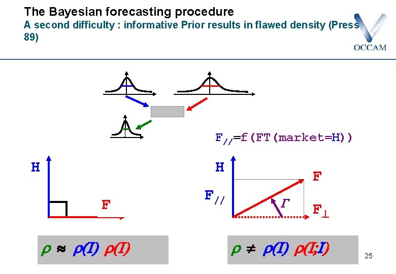
The Bayesian forecasting procedure A second difficulty : informative Prior results in flawed density (Press 89) F//=f(FT(market=H)) H H F (I) F// F F (I) (I; I) 25

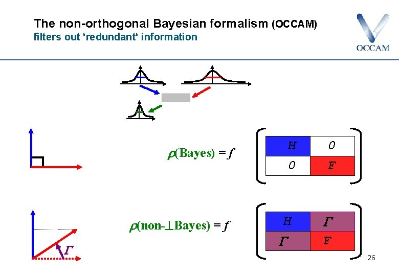
The non-orthogonal Bayesian formalism (OCCAM) filters out ‘redundant‘ information (Bayes) = f (non- Bayes) = f H 0 0 F H F 26

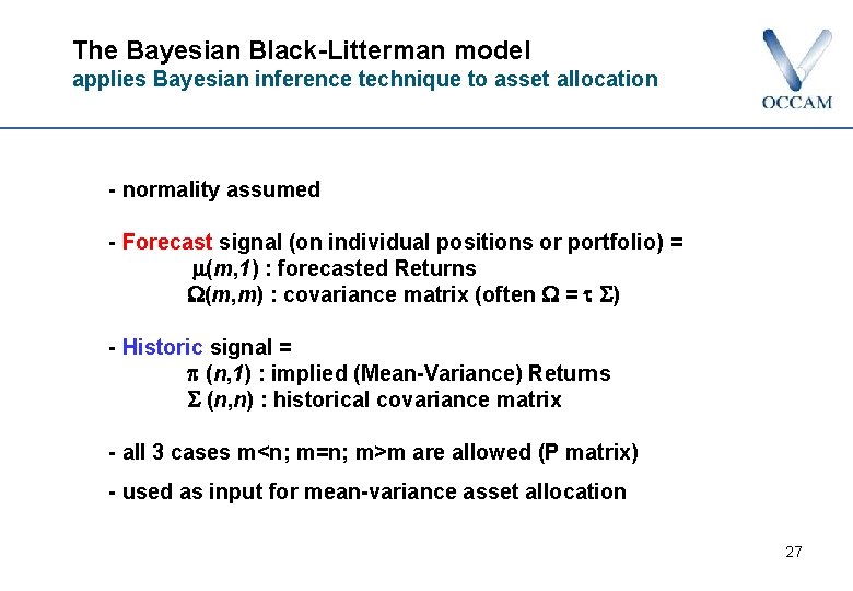
The Bayesian Black-Litterman model applies Bayesian inference technique to asset allocation - normality assumed - Forecast signal (on individual positions or portfolio) = (m, 1) : forecasted Returns (m, m) : covariance matrix (often = ) - Historic signal = (n, 1) : implied (Mean-Variance) Returns (n, n) : historical covariance matrix - all 3 cases m<n; m=n; m>m are allowed (P matrix) - used as input for mean-variance asset allocation 27

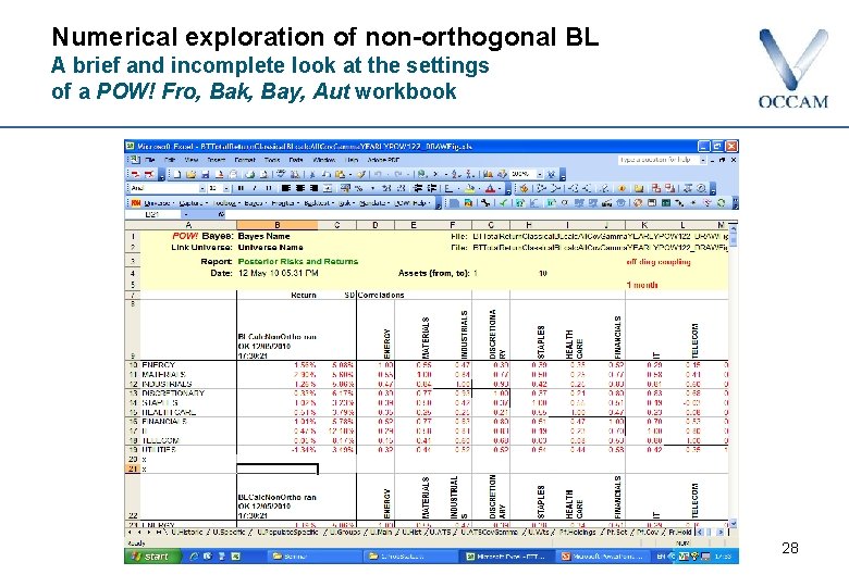
Numerical exploration of non-orthogonal BL A brief and incomplete look at the settings of a POW! Fro, Bak, Bay, Aut workbook 28

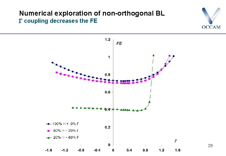
Numerical exploration of non-orthogonal BL coupling decreases the FE 29

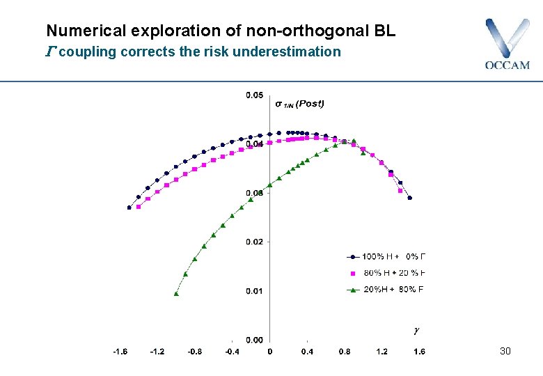
Numerical exploration of non-orthogonal BL coupling corrects the risk underestimation 30

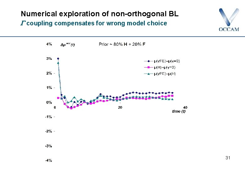
Numerical exploration of non-orthogonal BL coupling compensates for wrong model choice 31

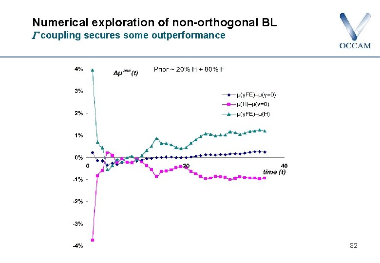
Numerical exploration of non-orthogonal BL coupling secures some outperformance 32

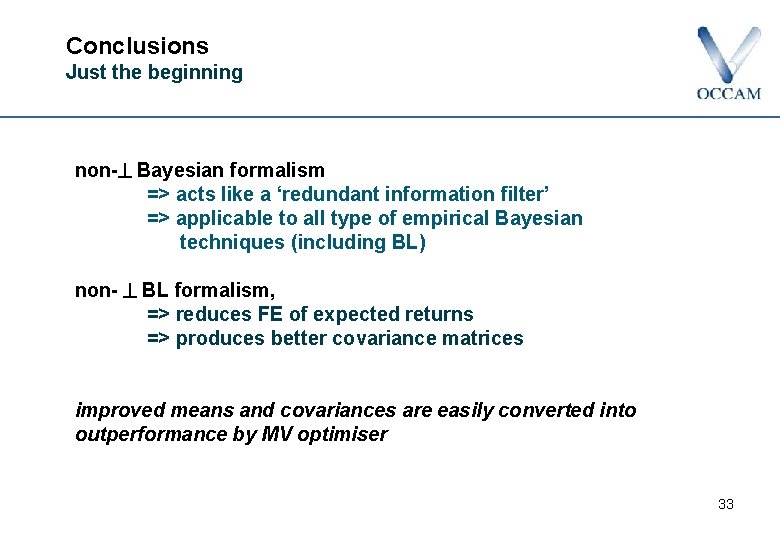
Conclusions Just the beginning non- Bayesian formalism => acts like a ‘redundant information filter’ => applicable to all type of empirical Bayesian techniques (including BL) non- BL formalism, => reduces FE of expected returns => produces better covariance matrices improved means and covariances are easily converted into outperformance by MV optimiser 33

Introducing POW! 1. 22 Compound Linear Constraints Protection against the unexpected 34

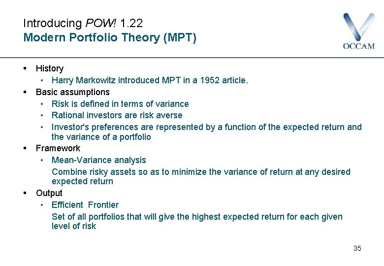
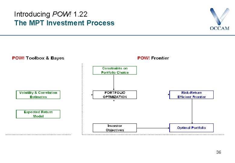
Introducing POW! 1. 22 Modern Portfolio Theory (MPT) § § History • Harry Markowitz introduced MPT in a 1952 article. Basic assumptions • Risk is defined in terms of variance • Rational investors are risk averse • Investor's preferences are represented by a function of the expected return and the variance of a portfolio Framework • Mean-Variance analysis Combine risky assets so as to minimize the variance of return at any desired expected return Output • Efficient Frontier Set of all portfolios that will give the highest expected return for each given level of risk 35

Introducing POW! 1. 22 The MPT Investment Process 36

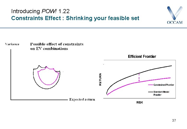
Introducing POW! 1. 22 Constraints Effect : Shrinking your feasible set 37

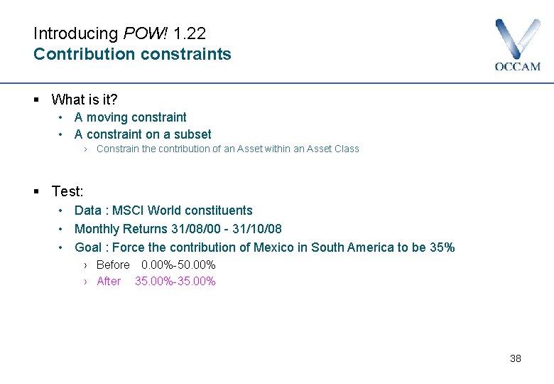
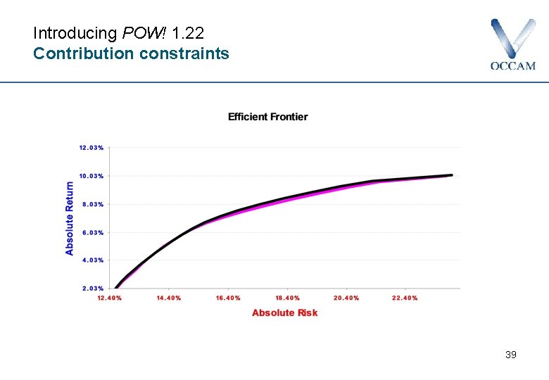
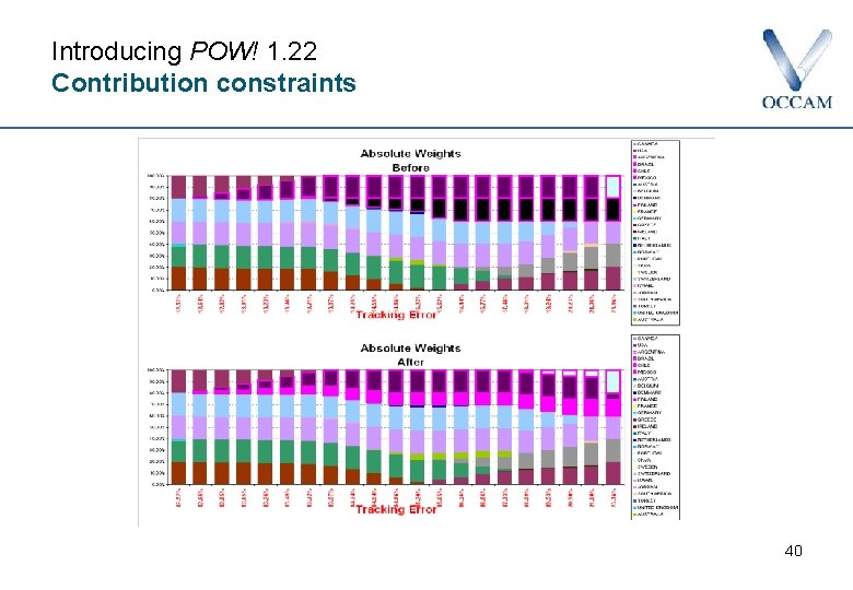
Introducing POW! 1. 22 Contribution constraints § What is it? • A moving constraint • A constraint on a subset › Constrain the contribution of an Asset within an Asset Class § Test: • Data : MSCI World constituents • Monthly Returns 31/08/00 - 31/10/08 • Goal : Force the contribution of Mexico in South America to be 35% › Before 0. 00%-50. 00% › After 35. 00%-35. 00% 38

Introducing POW! 1. 22 Contribution constraints 39

Introducing POW! 1. 22 Contribution constraints 40

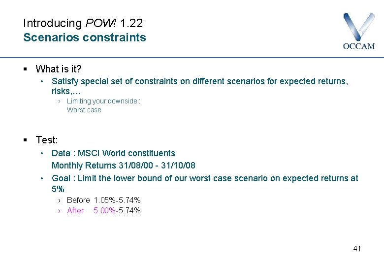
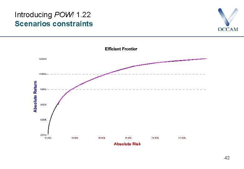
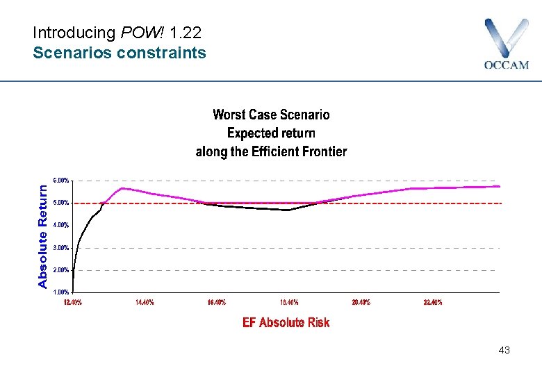
Introducing POW! 1. 22 Scenarios constraints § What is it? • Satisfy special set of constraints on different scenarios for expected returns, risks, … › Limiting your downside : Worst case § Test: • Data : MSCI World constituents Monthly Returns 31/08/00 - 31/10/08 • Goal : Limit the lower bound of our worst case scenario on expected returns at 5% › Before 1. 05%-5. 74% › After 5. 00%-5. 74% 41

Introducing POW! 1. 22 Scenarios constraints 42

Introducing POW! 1. 22 Scenarios constraints 43

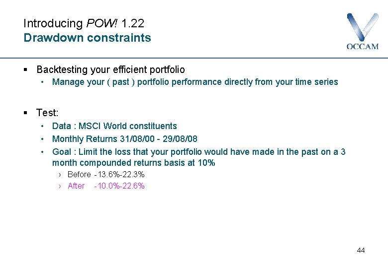
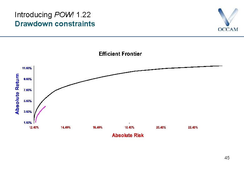
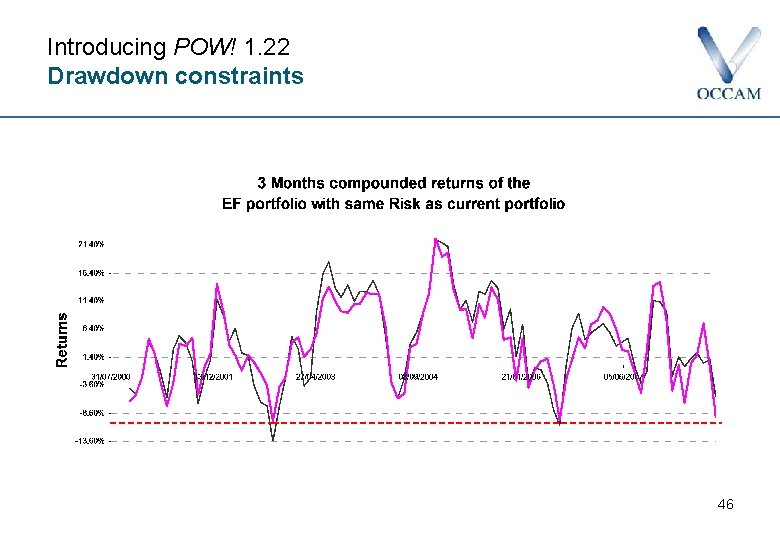
Introducing POW! 1. 22 Drawdown constraints § Backtesting your efficient portfolio • Manage your ( past ) portfolio performance directly from your time series § Test: • Data : MSCI World constituents • Monthly Returns 31/08/00 - 29/08/08 • Goal : Limit the loss that your portfolio would have made in the past on a 3 month compounded returns basis at 10% › Before -13. 6%-22. 3% › After -10. 0%-22. 6% 44

Introducing POW! 1. 22 Drawdown constraints 45

Introducing POW! 1. 22 Drawdown constraints 46

Introducing POW! 1. 22 What if history had been different? The balanced, block and calendar bootstrap 47

What if history had been different? The balanced, block and calendar bootstrap § The mean-variance optimisation problem to fix § The POW! Robust module § Is balanced bootstrap always appropriate ? § The block bootstrap and the calendar blocking § more on POW! TS facilities 48

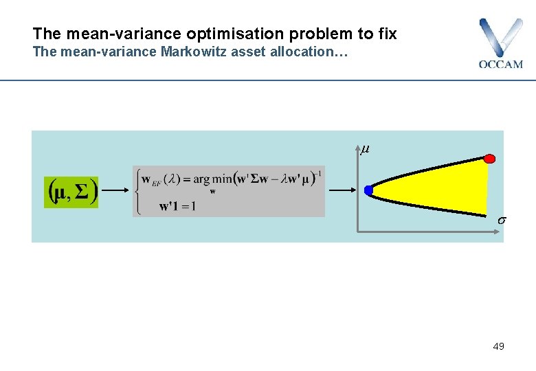
The mean-variance optimisation problem to fix The mean-variance Markowitz asset allocation… 49

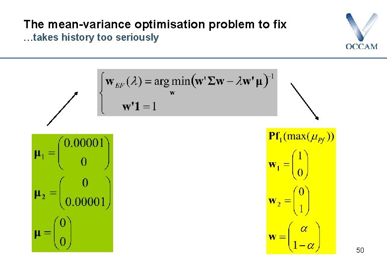
The mean-variance optimisation problem to fix …takes history too seriously 50

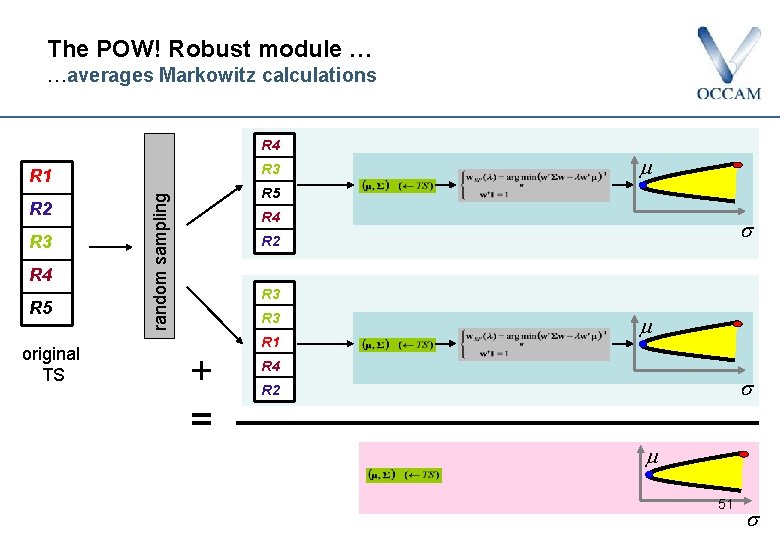
The POW! Robust module … …averages Markowitz calculations R 4 R 3 R 1 R 3 R 4 R 5 original TS R 5 random sampling R 2 R 4 R 2 R 3 + = R 1 R 4 R 2 51

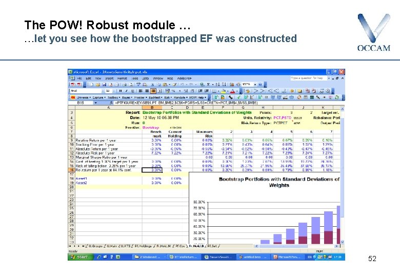
The POW! Robust module … …let you see how the bootstrapped EF was constructed 52

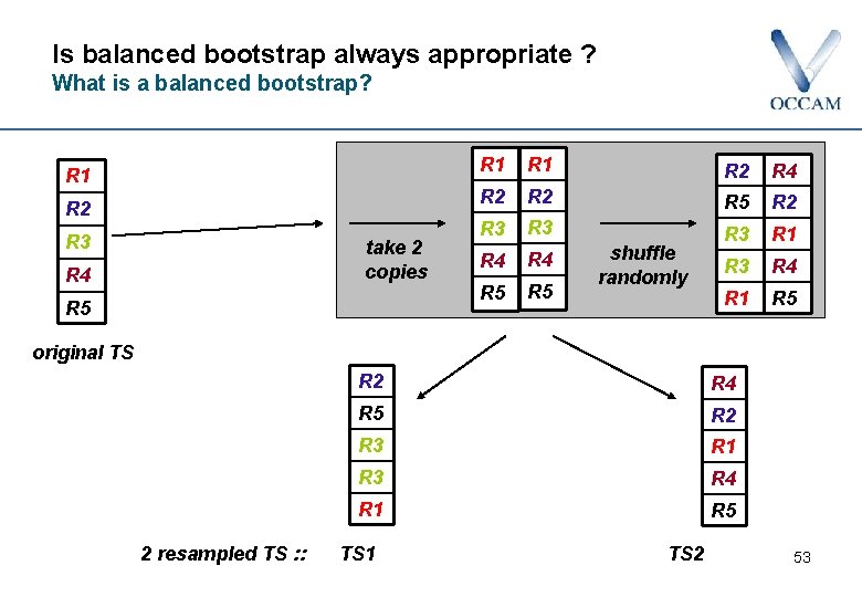
Is balanced bootstrap always appropriate ? What is a balanced bootstrap? R 1 R 2 R 3 take 2 copies R 4 R 5 R 1 R 2 R 4 R 2 R 5 R 2 R 3 R 3 R 1 R 4 R 3 R 4 R 5 R 1 R 5 shuffle randomly original TS 2 resampled TS : : R 2 R 4 R 5 R 2 R 3 R 1 R 3 R 4 R 1 R 5 TS 1 TS 2 53

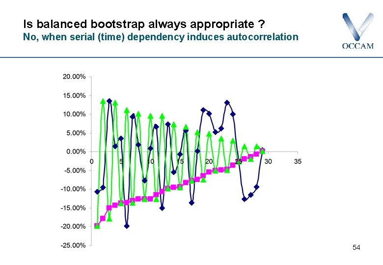
Is balanced bootstrap always appropriate ? No, when serial (time) dependency induces autocorrelation 54

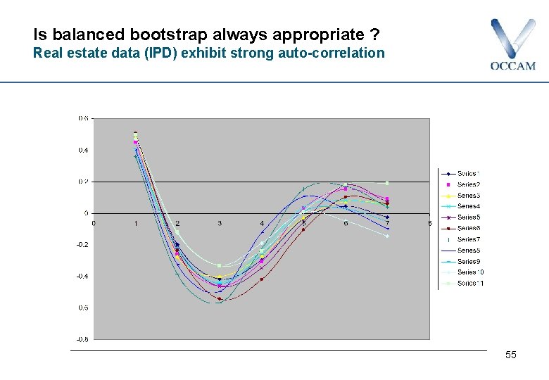
Is balanced bootstrap always appropriate ? Real estate data (IPD) exhibit strong auto-correlation 55

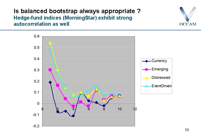
Is balanced bootstrap always appropriate ? Hedge-fund indices (Morning. Star) exhibit strong autocorrelation as well 56

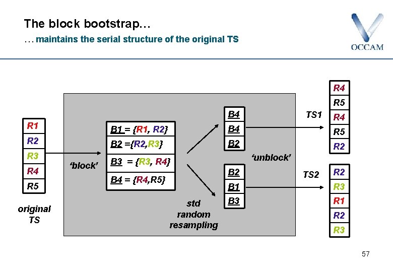
The block bootstrap… …maintains the serial structure of the original TS R 4 R 5 B 4 TS 1 R 4 R 1 B 1 = {R 1, R 2} B 4 R 2 R 5 B 2 ={R 2, R 3} B 2 R 3 R 4 R 5 original TS ‘block’ ‘unblock’ B 3 = {R 3, R 4} B 2 B 4 = {R 4, R 5} std random resampling TS 2 R 2 B 1 R 3 B 3 R 1 R 2 R 3 57

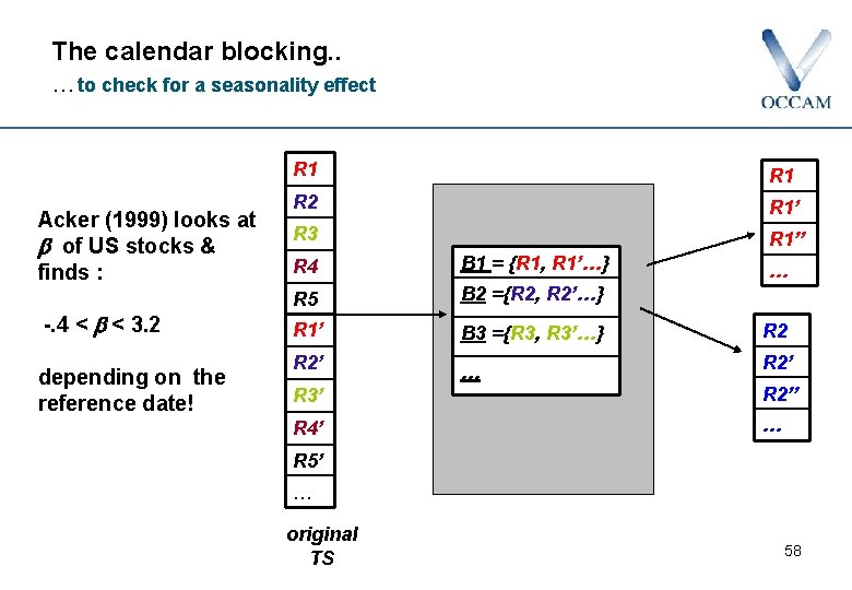
The calendar blocking. . …to check for a seasonality effect Acker (1999) looks at of US stocks & finds : -. 4 < < 3. 2 depending on the reference date! R 1 R 2 R 1’ R 3 R 1” R 4 B 1 = {R 1, R 1’…} R 5 B 2 ={R 2, R 2’…} R 1’ B 3 ={R 3, R 3’…} R 2’ … R 3’ R 2” R 4’ … R 5’ … original TS 58

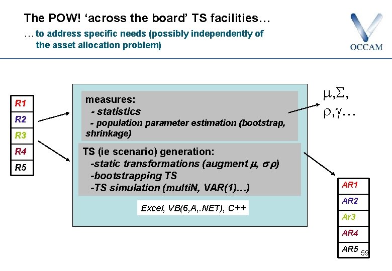
The POW! ‘across the board’ TS facilities… …to address specific needs (possibly independently of the asset allocation problem) R 1 R 2 R 3 R 4 R 5 measures: - statistics - population parameter estimation (bootstrap, shrinkage) TS (ie scenario) generation: -static transformations (augment , ) -bootstrapping TS -TS simulation (multi. N, VAR(1)…) Excel, VB(6, A, . NET), C++ , , , … AR 1 AR 2 Ar 3 AR 4 AR 5 59

Conclusions a few last observations § The problem of over-concentration of mean-variance portfolio is fixed by bootstrap resampling § The choice of the bootstrap method depends on the characteristics of the TS : balanced or block or calendar, or …? § TS facilities for those who need increase flexibility 60

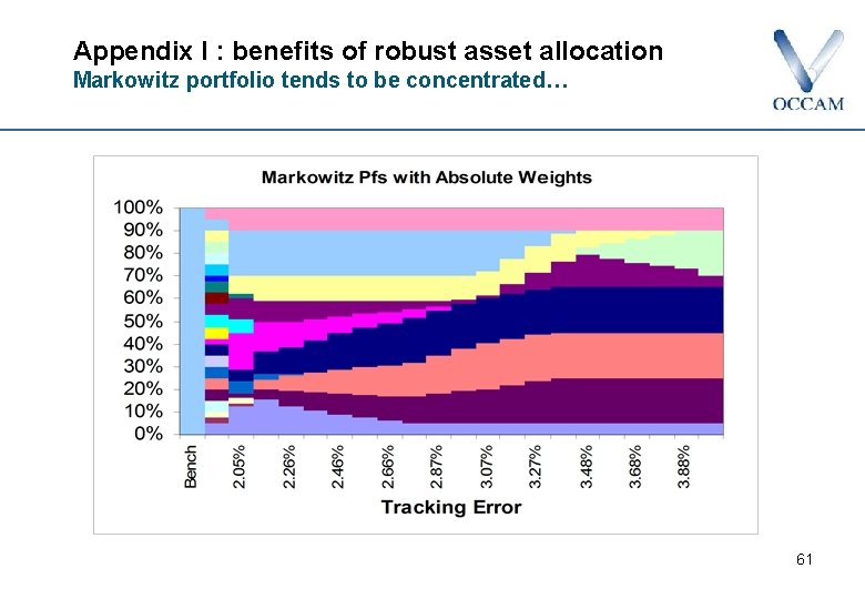
Appendix I : benefits of robust asset allocation Markowitz portfolio tends to be concentrated… 61

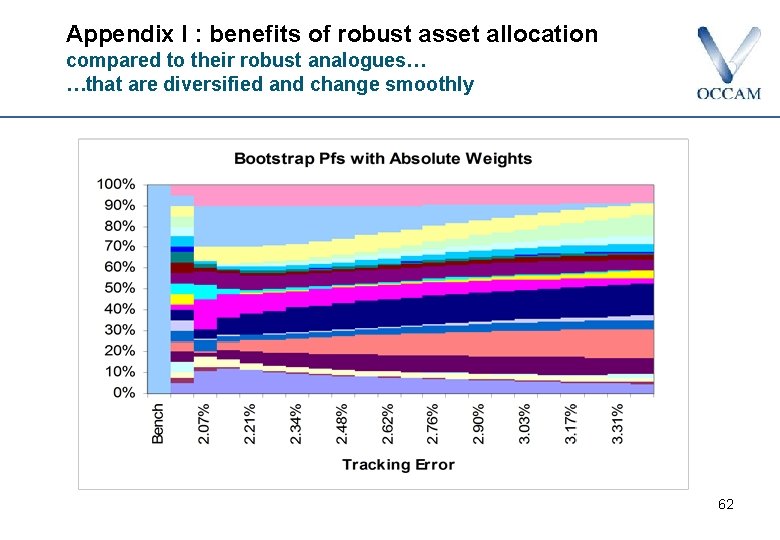
Appendix I : benefits of robust asset allocation compared to their robust analogues… …that are diversified and change smoothly 62

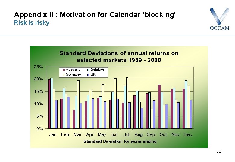
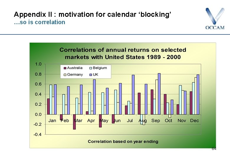
Appendix II : Motivation for Calendar ‘blocking’ Risk is risky 63

Appendix II : motivation for calendar ‘blocking’ …so is correlation 64

Introducing POW! 1. 22 Property is Different What can it teach us ? Direct or indirect: How can an investor decide ? 65

Property is different: what can it teach us ? Some questions: 1. What is the impact on portfolio risk of a) b) c) d) Number of stocks held ? Portfolio size ? Value-skewness (unequal lot sizes) ? How much alpha do I need to offset these impacts ? 2. What is the impact on the choice between direct and indirect of Portfolio size ? 66

The Tools for the Job § The Data • • • § The IPD monthly, quarterly and annual databases Individual IPD/IPF property risk data from Callender, Devaney and Sheahan 2007 (1995 -2004) The IPD AREF fund database The Model • The IPD / OCCAM UK Property model, developed by OCCAM in cooperation with IPD • Building on the work of • Ø Ø Bill Sharpe Guy Morrell Rice, R. Realistic Portfolio Analysis and Construction ERES 2007 67

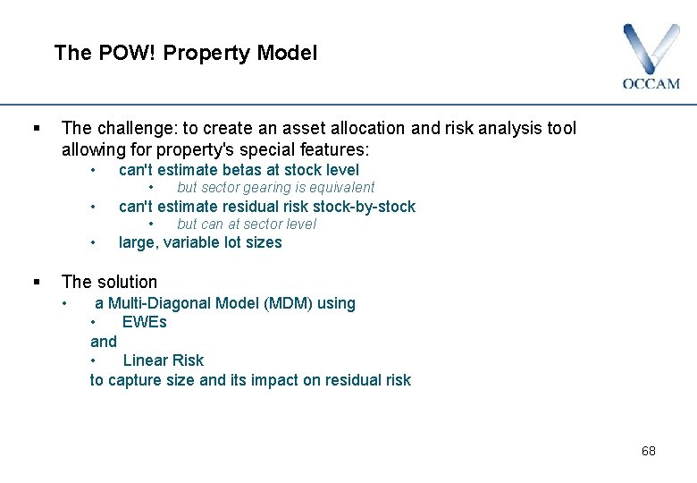
The POW! Property Model § The challenge: to create an asset allocation and risk analysis tool allowing for property's special features: • can't estimate betas at stock level • • can't estimate residual risk stock-by-stock • • § but sector gearing is equivalent but can at sector level large, variable lot sizes The solution • a Multi-Diagonal Model (MDM) using • EWEs and • Linear Risk to capture size and its impact on residual risk 68

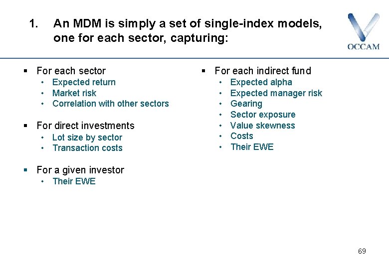
1. An MDM is simply a set of single-index models, one for each sector, capturing: § For each sector • Expected return • Market risk • Correlation with other sectors § For direct investments • Lot size by sector • Transaction costs § For each indirect fund • • Expected alpha Expected manager risk Gearing Sector exposure Value skewness Costs Their EWE § For a given investor • Their EWE 69

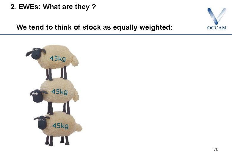
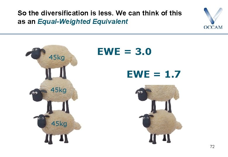
2. EWEs: What are they ? We tend to think of stock as equally weighted: 45 kg 70

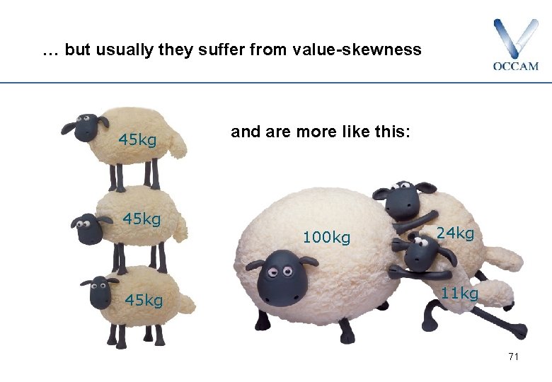
… but usually they suffer from value-skewness 45 kg and are more like this: 100 kg 24 kg 11 kg 71

So the diversification is less. We can think of this as an Equal-Weighted Equivalent 45 kg EWE = 3. 0 EWE = 1. 7 45 kg 72

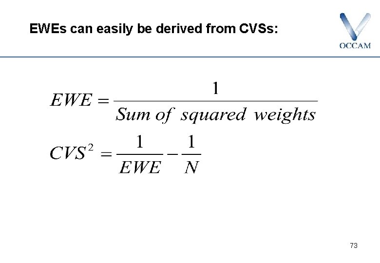
EWEs can easily be derived from CVSs: 73

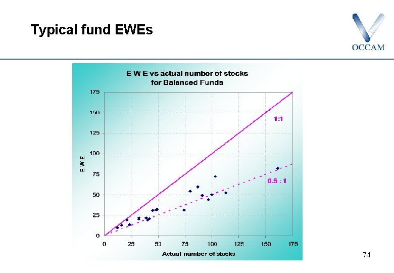
Typical fund EWEs 74

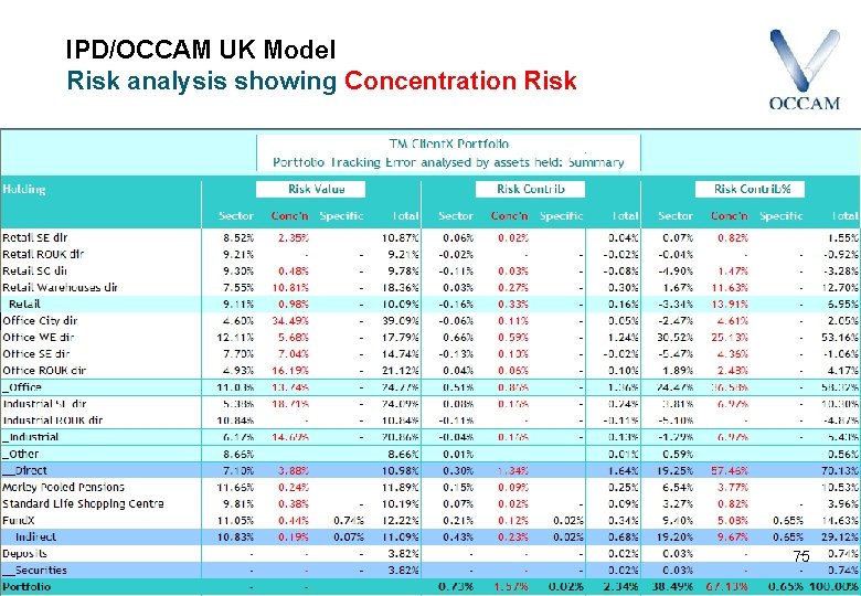
IPD/OCCAM UK Model Risk analysis showing Concentration Risk 75

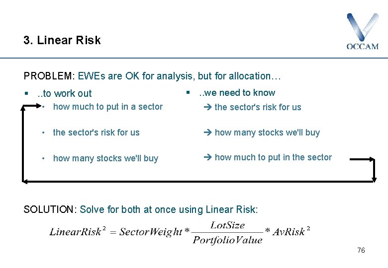
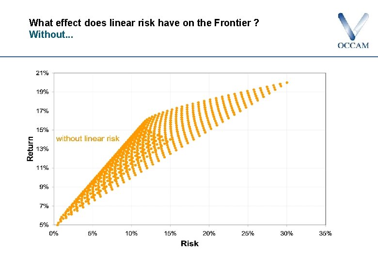
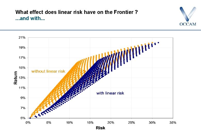
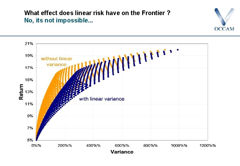
3. Linear Risk PROBLEM: EWEs are OK for analysis, but for allocation… §. . to work out §. . we need to know • how much to put in a sector è the sector's risk for us • the sector's risk for us è how many stocks we'll buy • how many stocks we'll buy è how much to put in the sector SOLUTION: Solve for both at once using Linear Risk: 76

So now let’s look at allocation and get the Optimiser to answer our questions 77

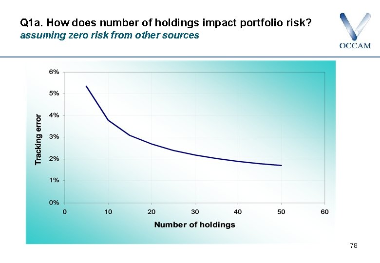
Q 1 a. How does number of holdings impact portfolio risk? assuming zero risk from other sources 78

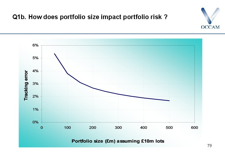
Q 1 b. How does portfolio size impact portfolio risk ? 79

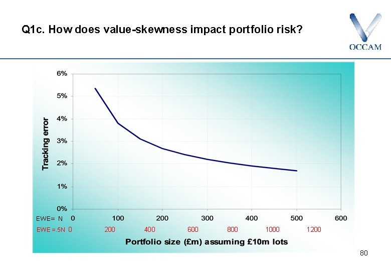
Q 1 c. How does value-skewness impact portfolio risk? EWE= N EWE =. 5 N 0 200 400 600 800 1000 1200 80

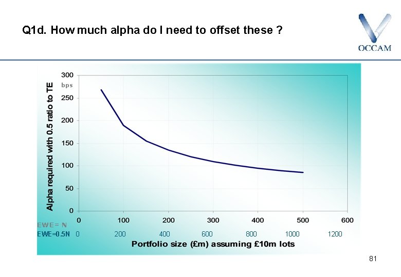
Q 1 d. How much alpha do I need to offset these ? bps EWE= N EWE=0. 5 N 0 200 400 600 800 1000 1200 81

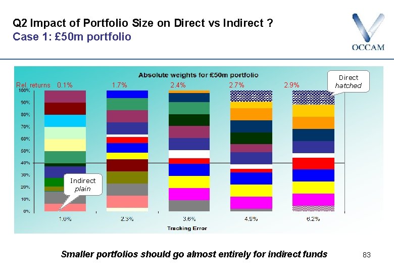
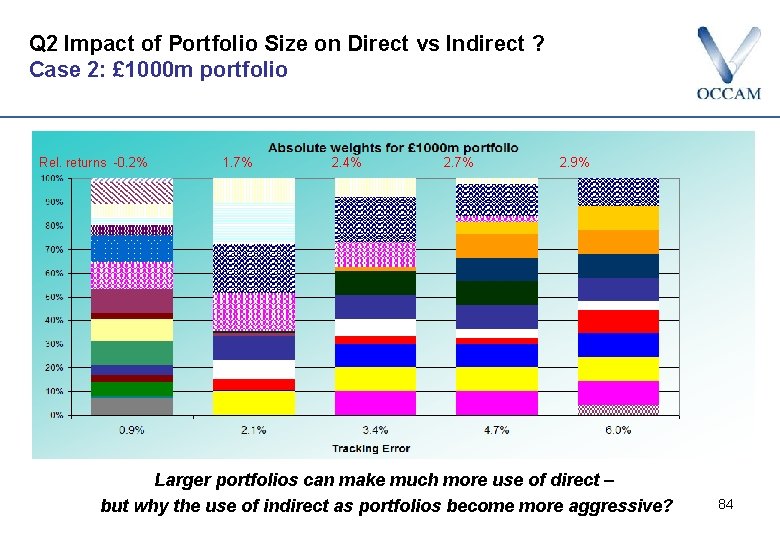
Q 1. Conclusion and Lesson § Size brings increased diversification potential § Small funds require enormous alpha to make Direct worthwhile • especially if they are skewed § Much better to hold an indirect stake in a fund • even if it has negative alpha • provided management fees are reasonable ! § What can Property teach us ? • The same applies to not-so-high-net-worth investors in equities etc 82

Q 2 Impact of Portfolio Size on Direct vs Indirect ? Case 1: £ 50 m portfolio Rel. returns 0. 1% 1. 7% 2. 4% 2. 7% 2. 9% Direct hatched Indirect plain Smaller portfolios should go almost entirely for indirect funds 83

Q 2 Impact of Portfolio Size on Direct vs Indirect ? Case 2: £ 1000 m portfolio Rel. returns -0. 2% 1. 7% 2. 4% 2. 7% 2. 9% Larger portfolios can make much more use of direct – but why the use of indirect as portfolios become more aggressive? 84

What effect does linear risk have on the Frontier ? Without. . .

What effect does linear risk have on the Frontier ? . . . and with. . .

What effect does linear risk have on the Frontier ? No, its not impossible. . .

Where next ? § The MDM approach can be applied: • on a custom or DIY basis to • different UK segmentations, eg age of build, floor area • in the IPD/OCCAM Global Property Model to • global portfolios (with/without currency hedging • forthcoming • to individual countries outside the UK • You name it ! § Bells and whistles can be added, such as • currencies • value creep • correlated residuals and managers • apply Ledoit shrinkage to condition the matrix • etc

Introducing POW! 1. 22 Guest Speaker: Malcolm Frodsham Director of Research, IPD Portfolio and market probability-adjusted cash-flow modelling with PAC-M 89

Portfolio and Market probabilityadjusted Cash Flow Modelling with PAC-M On the pulse of the property world OCCAM Seminar – 14 th May 2010

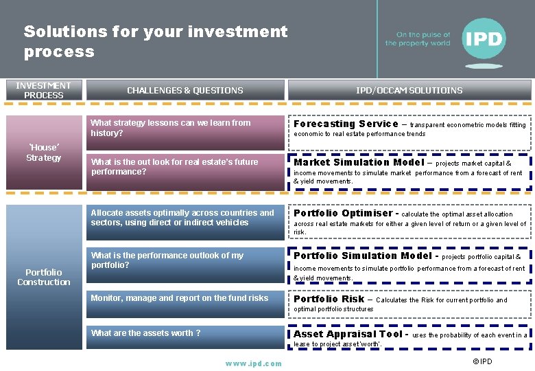
Solutions for your investment process INVESTMENT PROCESS ‘House’ Strategy Portfolio Construction CHALLENGES & QUESTIONS IPD/OCCAM SOLUTIOINS What strategy lessons can we learn from history? Forecasting Service – What is the out look for real estate’s future performance? Market Simulation Model – Allocate assets optimally across countries and sectors, using direct or indirect vehicles Portfolio Optimiser - calculate the optimal asset allocation What is the performance outlook of my portfolio? Portfolio Simulation Model - Monitor, manage and report on the fund risks Portfolio Risk – transparent econometric models fitting economic to real estate performance trends projects market capital & income movements to simulate market performance from a forecast of rent & yield movements. across real estate markets for either a given level of return or a given level of risk. projects portfolio capital & income movements to simulate portfolio performance from a forecast of rent & yield movements. Calculates the Risk for current portfolio and optimal portfolio structures Asset Appraisal Tool - What are the assets worth ? uses the probability of each event in a lease to project asset ‘worth’. www. ipd. com © IPD

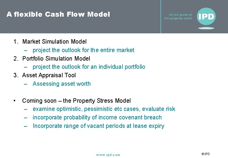
A flexible Cash Flow Model 1. Market Simulation Model – project the outlook for the entire market 2. Portfolio Simulation Model – project the outlook for an individual portfolio 3. Asset Appraisal Tool – Assessing asset worth • Coming soon – the Property Stress Model – examine optimistic, pessimistic etc cases, evaluate risk – incorporate probability of income covenant breach – Incorporate range of vacant periods at lease expiry www. ipd. com © IPD

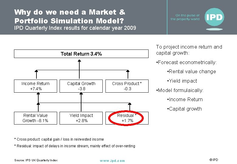
Why do we need a Market & Portfolio Simulation Model? IPD Quarterly Index results for calendar year 2009 To project income return and capital growth: Total Return 3. 4% • Forecast econometrically: • Rental value change Income Return +7. 4% Capital Growth -3. 8 Cross Product * -0. 3 • Yield impact • Model formulaically: • Income Return • Capital growth Rental Value Growth -8. 1% Yield Impact +2. 8% Residual * +1. 7% * Cross product: capital gain / loss in reinvested income * Residual: impact of delays in income stream, mainly effect of over-renting Source: IPD UK Quarterly Index www. ipd. com © IPD

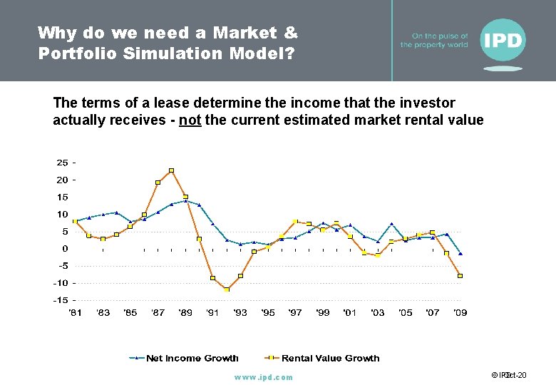
Why do we need a Market & Portfolio Simulation Model? The terms of a lease determine the income that the investor actually receives - not the current estimated market rental value www. ipd. com © IPD Oct-20

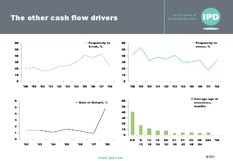
The other cash flow drivers www. ipd. com © IPD

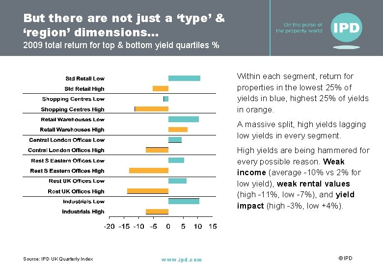
But there are not just a ‘type’ & ‘region’ dimensions… 2009 total return for top & bottom yield quartiles % Within each segment, return for properties in the lowest 25% of yields in blue, highest 25% of yields in orange. A massive split, high yields lagging low yields in every segment. High yields are being hammered for every possible reason. Weak income (average -10% vs 2% for low yield), weak rental values (high -11%, low -7%), and yield impact (high -3%, low +4%). Source: IPD UK Quarterly Index www. ipd. com © IPD

A flexible Cash Flow Model 1. Market Simulation Model – project the outlook for the entire market 2. Portfolio Simulation Model – project the outlook for an individual portfolio – Value opportunities can be highlighted: – Enables performance by asset quality to be added to a House View – Forecasts of rental value change can be extended to forecasts of leasing variables www. ipd. com © IPD

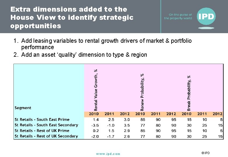
Extra dimensions added to the House View to identify strategic opportunities 1. Add leasing variables to rental growth drivers of market & portfolio performance 2. Add an asset ‘quality’ dimension to type & region www. ipd. com © IPD

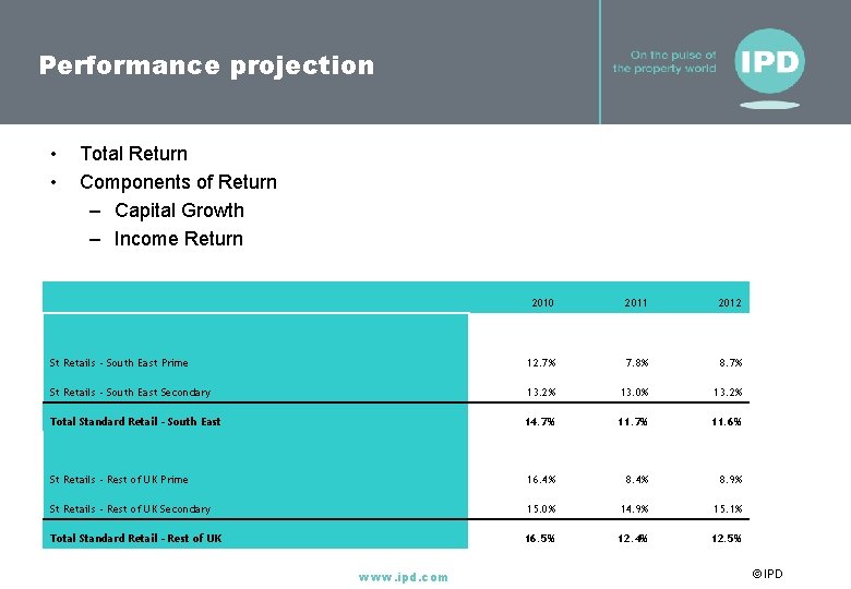
Performance projection • • Total Return Components of Return – Capital Growth – Income Return 2010 2011 2012 St Retails - South East Prime 12. 7% 7. 8% 8. 7% St Retails - South East Secondary 13. 2% 13. 0% 13. 2% Total Standard Retail - South East 14. 7% 11. 6% St Retails - Rest of UK Prime 16. 4% 8. 9% St Retails - Rest of UK Secondary 15. 0% 14. 9% 15. 1% Total Standard Retail - Rest of UK 16. 5% 12. 4% 12. 5% www. ipd. com © IPD

Income projection www. ipd. com © IPD

A flexible Cash Flow Model to identify ‘worth’ 1. Market Simulation Model – project the outlook for the entire market 2. Portfolio Simulation Model – project the outlook for an individual portfolio 3. Asset Appraisal Tool – Assessing asset worth • • There is inefficiency in market pricing as valuations are driven by short-cut DCF techniques Asset appraisal should incorporate changes in the outlook for the fundamental drivers of asset worth before they are picked up in changes in market pricing – Changes in lease lengths, propensity to renew, propensity to break, average vacancy period – How these variables vary over the life of an asset www. ipd. com © IPD

The physical characteristics of assets deteriorate over time and diminish the utility of the building Causes of obsolescence: i. Deterioration of the physical structure ii. Aesthetic look of the building; iii. Compliance with current law (such as compliance with accessibility for the disabled) iv. Functional layout, such as raised floors or open plan layout. www. ipd. com © IPD

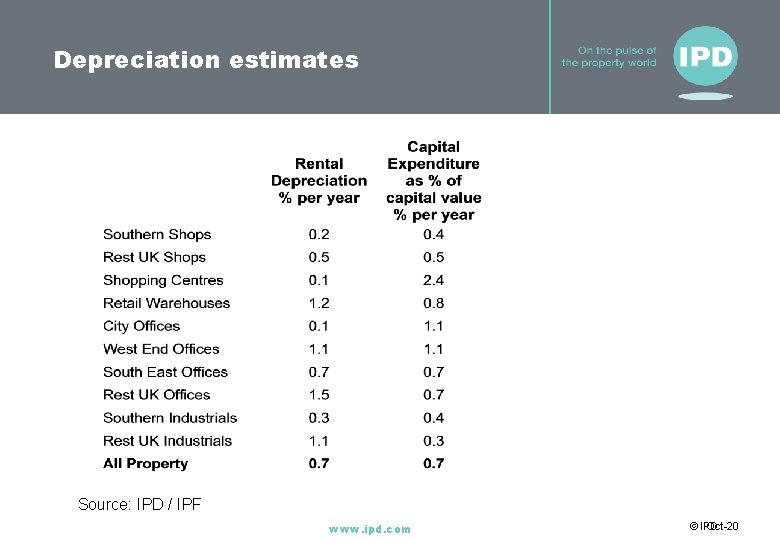
Depreciation estimates Source: IPD / IPF www. ipd. com © IPD Oct-20

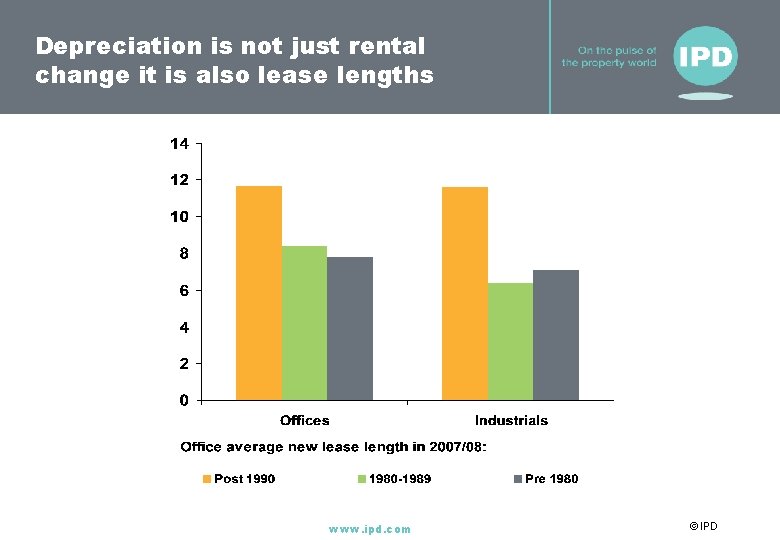
Depreciation is not just rental change it is also lease lengths www. ipd. com © IPD

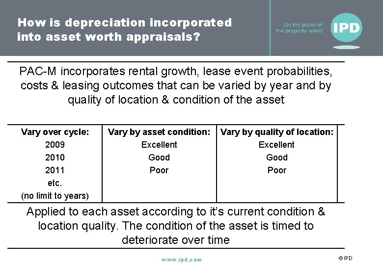
How is depreciation incorporated into asset worth appraisals? PAC-M incorporates rental growth, lease event probabilities, costs & leasing outcomes that can be varied by year and by quality of location & condition of the asset Vary over cycle: 2009 2010 2011 etc. (no limit to years) Vary by asset condition: Excellent Good Poor Vary by quality of location: Excellent Good Poor Applied to each asset according to it’s current condition & location quality. The condition of the asset is timed to deteriorate over time www. ipd. com © IPD

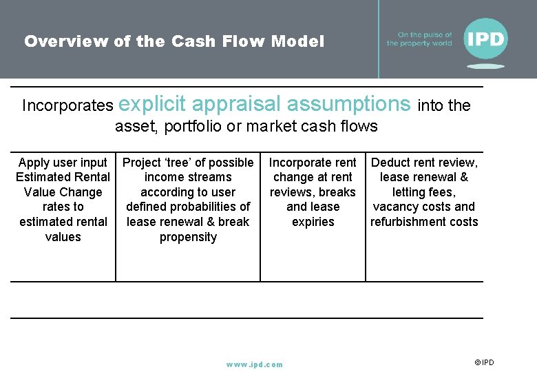
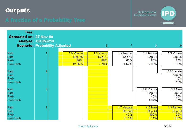
Overview of the Cash Flow Model Incorporates explicit appraisal assumptions into the asset, portfolio or market cash flows Apply user input Project ‘tree’ of possible Estimated Rental income streams Value Change according to user rates to defined probabilities of estimated rental lease renewal & break values propensity Incorporate rent change at rent reviews, breaks and lease expiries www. ipd. com Deduct rent review, lease renewal & letting fees, vacancy costs and refurbishment costs © IPD

Outputs A fraction of a Probability Tree www. ipd. com © IPD

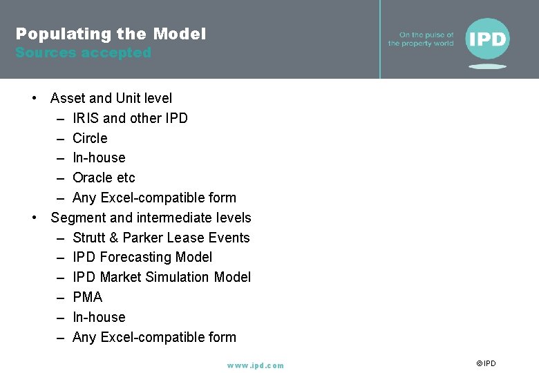
Populating the Model Sources accepted • Asset and Unit level – IRIS and other IPD – Circle – In-house – Oracle etc – Any Excel-compatible form • Segment and intermediate levels – Strutt & Parker Lease Events – IPD Forecasting Model – IPD Market Simulation Model – PMA – In-house – Any Excel-compatible form www. ipd. com © IPD

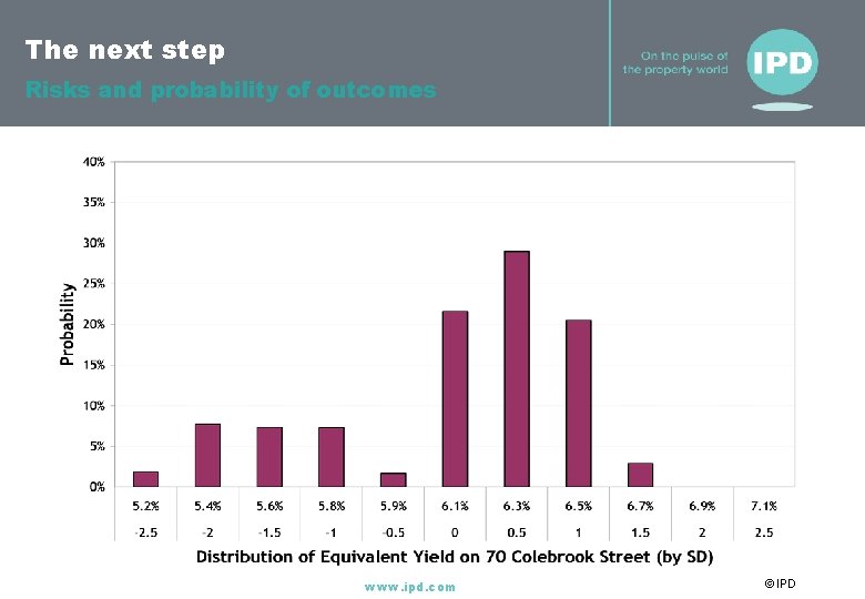
The next step Risks and probability of outcomes www. ipd. com © IPD

Thank you for your time IPD 1 St. John’s Lane London, EC 1 M 4 BL United Kingdom Tel: +44 (0)20 7336 9200 Email: marketing@ipd. com Web: www. ipd. com Intellectual Property Rights and use of IPD statistics as benchmarks Whether in the public domain or otherwise, IPD's statistics are the intellectual property of Investment Property Databank Limited. It is not permissible to use data drawn from this presentation as benchmarks. © Investment Property Databank Limited (IPD) 2008. Database Right, Investment Property Databank Limited (IPD) 2008. All rights conferred by law of copyright and by virtue of international conventions are reserved by IPD www. ipd. com © IPD

Introducing POW! 1. 22 Flash Presentations 111

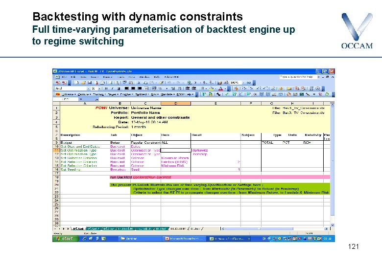
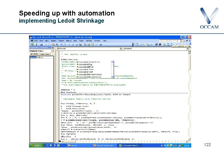
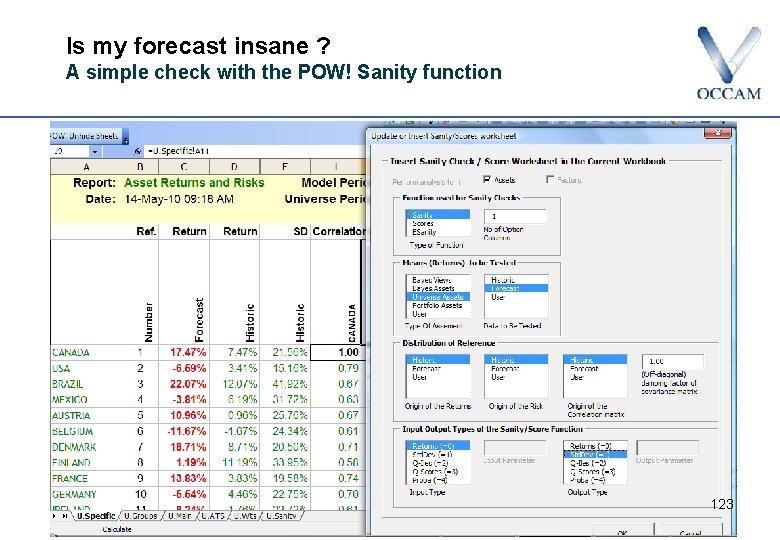
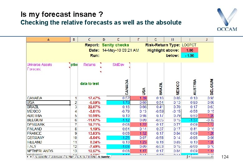
Introducing POW! 1. 22 Flash Presentations § Return attribution: Mirabelli or Russell ? § Efficient allocation and reporting for multiple portfolios § Speeding up with automation: implementing Ledoit shrinkage § Backtesting with dynamic constraints § Is my forecast insane ? § Coherent risk budgeting 112

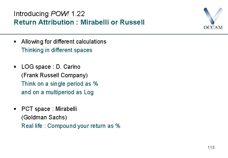
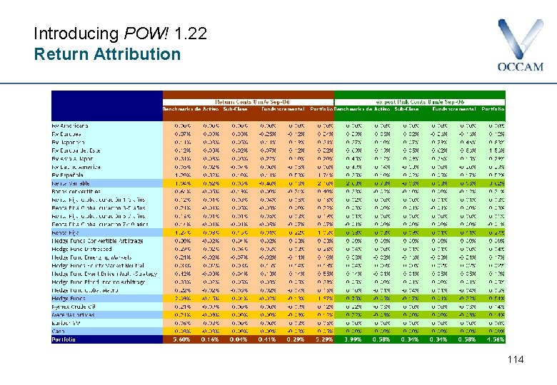
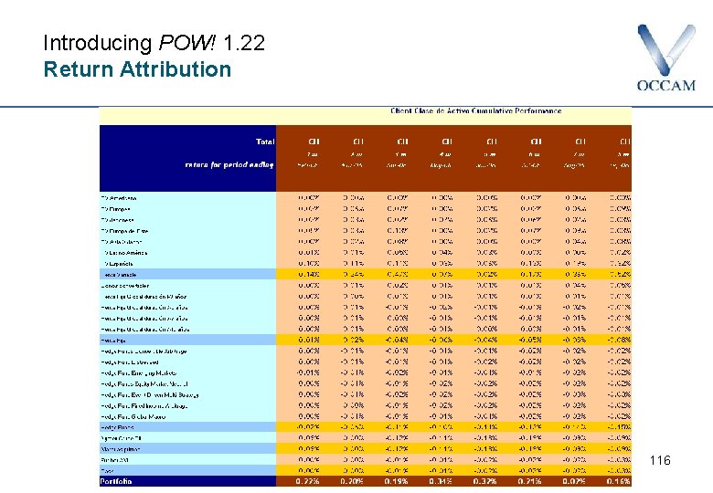
Introducing POW! 1. 22 Return Attribution : Mirabelli or Russell § Allowing for different calculations Thinking in different spaces § LOG space : D. Carino (Frank Russell Company) Think on a single period as % and on a multiperiod as Log § PCT space : Mirabelli (Goldman Sachs) Real life : Compound your return as % 113

Introducing POW! 1. 22 Return Attribution 114

Introducing POW! 1. 22 Return Attribution 115

Introducing POW! 1. 22 Return Attribution 116

Introducing POW! 1. 22 Return Attribution 117

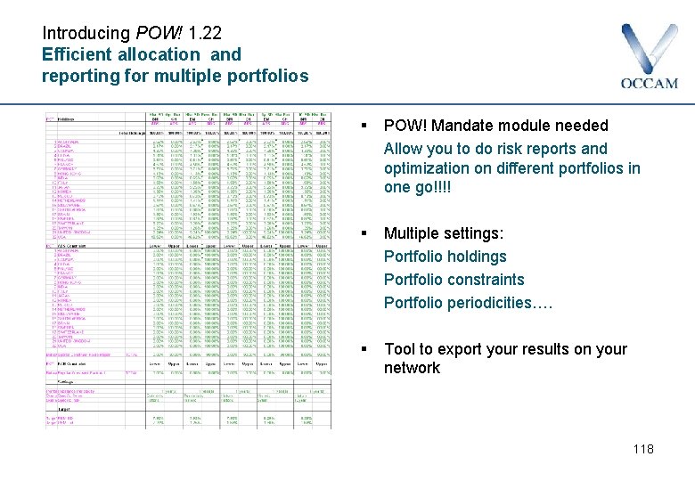
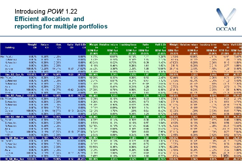
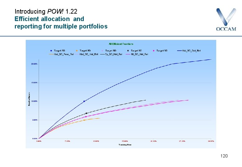
Introducing POW! 1. 22 Efficient allocation and reporting for multiple portfolios § POW! Mandate module needed Allow you to do risk reports and optimization on different portfolios in one go!!!! § Multiple settings: Portfolio holdings Portfolio constraints Portfolio periodicities…. § Tool to export your results on your network 118

Introducing POW! 1. 22 Efficient allocation and reporting for multiple portfolios 119

Introducing POW! 1. 22 Efficient allocation and reporting for multiple portfolios 120

Backtesting with dynamic constraints Full time-varying parameterisation of backtest engine up to regime switching 121

Speeding up with automation implementing Ledoit Shrinkage 122

Is my forecast insane ? A simple check with the POW! Sanity function 123

Is my forecast insane ? Checking the relative forecasts as well as the absolute 124

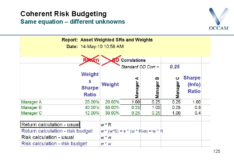
Coherent Risk Budgeting Same equation – different unknowns 125

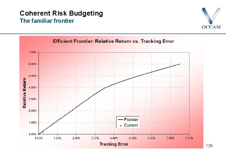
Coherent Risk Budgeting The familiar frontier 126

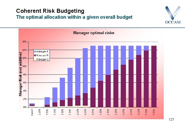
Coherent Risk Budgeting The optimal allocation within a given overall budget 127

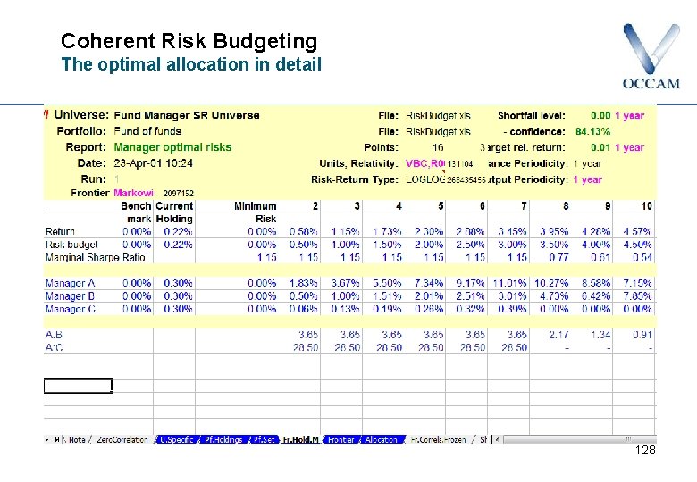
Coherent Risk Budgeting The optimal allocation in detail 128

Introducing POW! 1. 22 Programme for today § Overview and catch-up on the POW! Framework § Using maths to solve problems • Missing data: how do I fill the gaps ? • What do I do if my forecasts are partly based on history ? § Using algorithms to do the hard work • Drawdown constraints, alternative scenarios and other belts and braces • Ensuring portfolios are robust under different histories: the bootstrap § Learning from property is different, and what it can teach us • Direct or indirect ? How can an investor decide ? › POW! applied to the IPD / OCCAM UK and Global property models • Probability-adjusted cash-flow modelling with PAC-M § Flash presentations § Questions 129

For more information, please do not hesitate to contact us: OCCAM Financial Technology 220 Tower Bridge Road London SE 1 2 UP United Kingdom +44 (0) 20 7357 0400 office@occamsrazor. com www. occamsrazor. com