ICT TECHNOLOGIES IN WILDLAND FIRES MODELLING FOR TEST

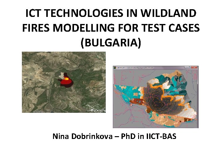
ICT TECHNOLOGIES IN WILDLAND FIRES MODELLING FOR TEST CASES (BULGARIA) Nina Dobrinkova – Ph. D in IICT-BAS

In this presentation … 1) Data availability for the test cases in Bulgaria 2) Calibrations with the available models 3) Simulations 4) Conclusions

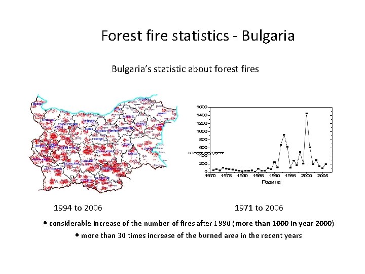
Forest fire statistics - Bulgaria’s statistic about forest fires 1994 to 2006 1971 to 2006 • considerable increase of the number of fires after 1990 (more than 1000 in year 2000) • more than 30 times increase of the burned area in the recent years

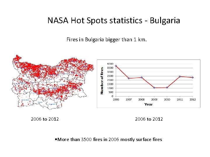
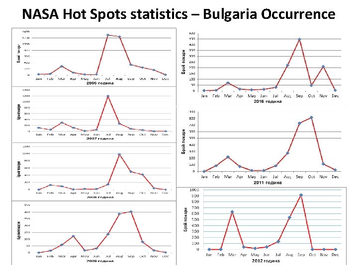
NASA Hot Spots statistics - Bulgaria Fires in Bulgaria bigger than 1 km. 2006 to 2012 • More than 3500 fires in 2006 mostly surface fires

NASA Hot Spots statistics – Bulgaria Occurrence

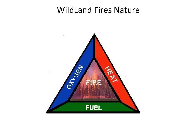
Wild. Land Fires Nature

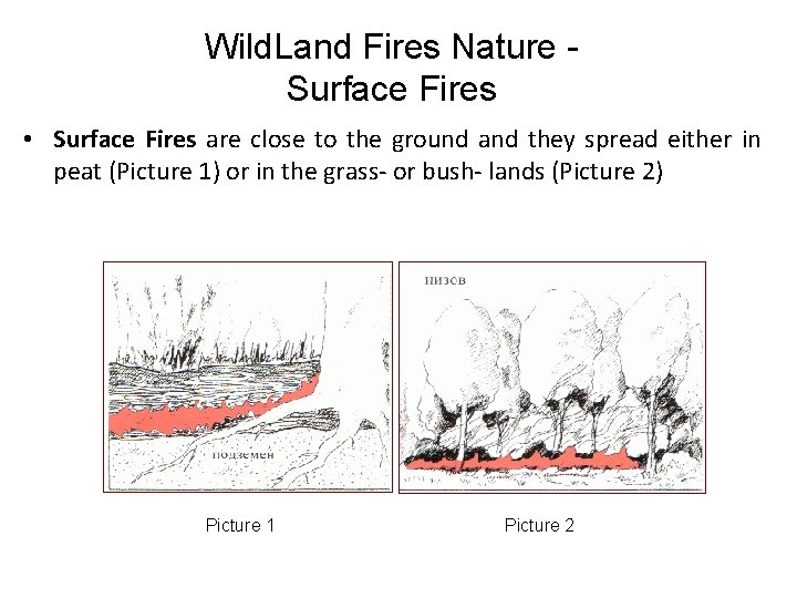
Wild. Land Fires Nature Surface Fires • Surface Fires are close to the ground and they spread either in peat (Picture 1) or in the grass- or bush- lands (Picture 2) Picture 1 Picture 2

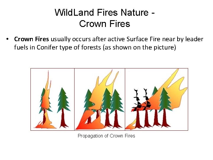
Wild. Land Fires Nature Crown Fires • Crown Fires usually occurs after active Surface Fire near by leader fuels in Conifer type of forests (as shown on the picture) Propagation of Crown Fires

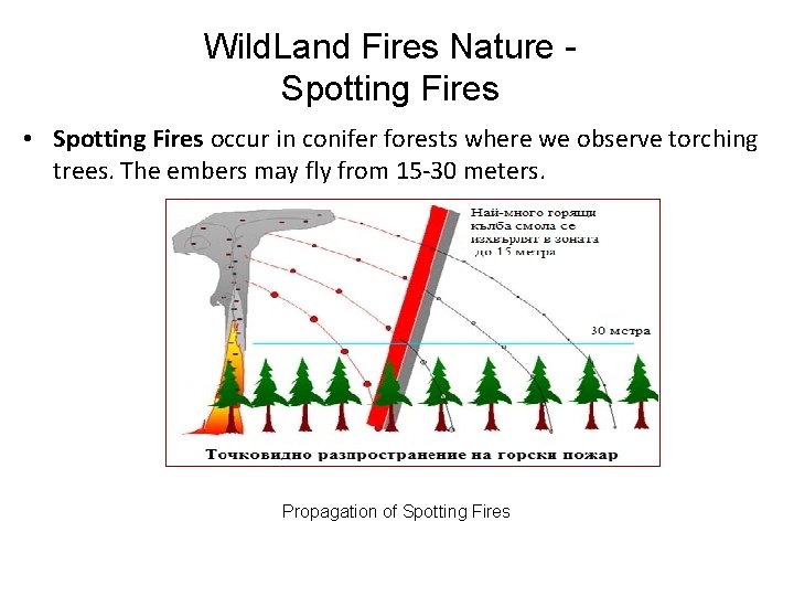
Wild. Land Fires Nature Spotting Fires • Spotting Fires occur in conifer forests where we observe torching trees. The embers may fly from 15 -30 meters. Propagation of Spotting Fires

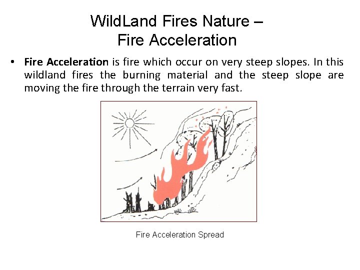
Wild. Land Fires Nature – Fire Acceleration • Fire Acceleration is fire which occur on very steep slopes. In this wildland fires the burning material and the steep slope are moving the fire through the terrain very fast. Fire Acceleration Spread

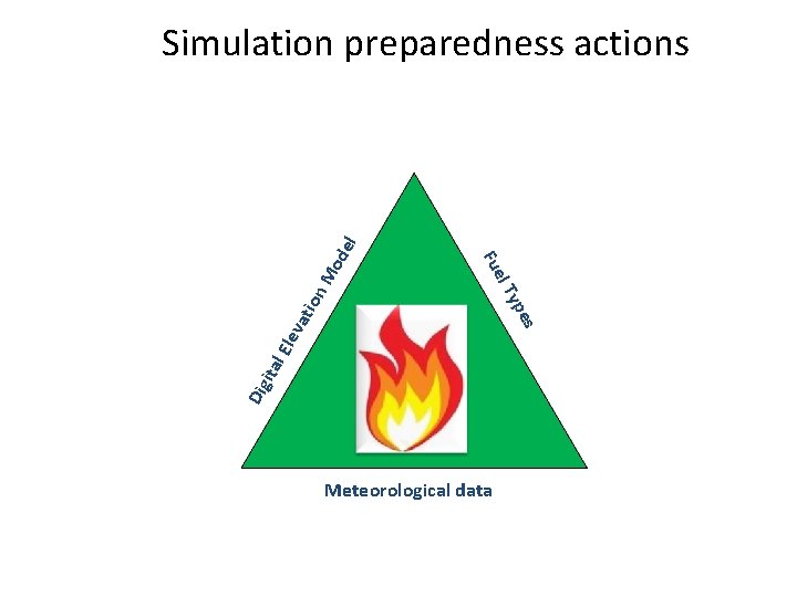
Mo on ati Dig it al E lev s pe Ty el Fu de l Simulation preparedness actions Meteorological data

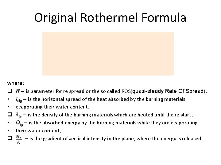
Original Rothermel Formula where: q R – is parameter for re spread or the so called ROS(quasi-steady Rate Of Spread), • Ixig – is the horizontal spread of the heat absorbed by the burning materials • evaporating their water content, q – is the density of the burning materials which are heated until the re start, • Qig – is the absorbed energy by the burning materials while they are evaporating • their water content, q – is the gradient of vertical intensity in the plane, where the energy is released.

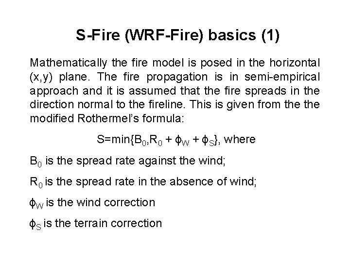
S-Fire (WRF-Fire) basics (1) Mathematically the fire model is posed in the horizontal (x, y) plane. The fire propagation is in semi-empirical approach and it is assumed that the fire spreads in the direction normal to the fireline. This is given from the modified Rothermel’s formula: S=min{B 0, R 0 + ɸW + ɸS}, where B 0 is the spread rate against the wind; R 0 is the spread rate in the absence of wind; ɸW is the wind correction ɸS is the terrain correction

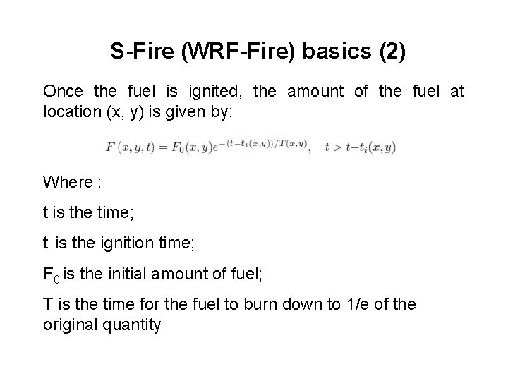
S-Fire (WRF-Fire) basics (2) Once the fuel is ignited, the amount of the fuel at location (x, y) is given by: Where : t is the time; ti is the ignition time; F 0 is the initial amount of fuel; T is the time for the fuel to burn down to 1/e of the original quantity

S-Fire (WRF-Fire) basics (3) From slides (1) and (2) we have idea about the plane, where the fire will spread and the fuel which we want to ignited, but we also need the heat flux, which is inserted as the time derivative of the temperature, while the latent heat flux as the time derivative of water vapor concentration. This scheme is required because atmospheric models with explicit time stepping, such as WRF, do not support flux boundary conditions.

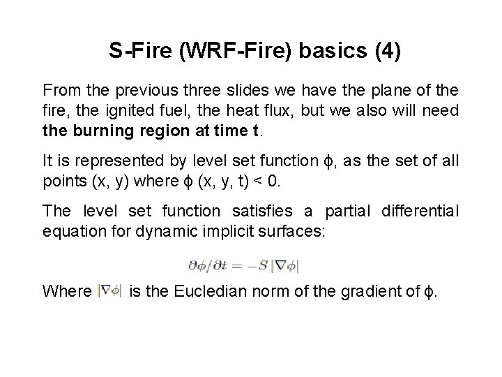
S-Fire (WRF-Fire) basics (4) From the previous three slides we have the plane of the fire, the ignited fuel, the heat flux, but we also will need the burning region at time t. It is represented by level set function ɸ, as the set of all points (x, y) where ɸ (x, y, t) < 0. The level set function satisfies a partial differential equation for dynamic implicit surfaces: Where is the Eucledian norm of the gradient of ɸ.

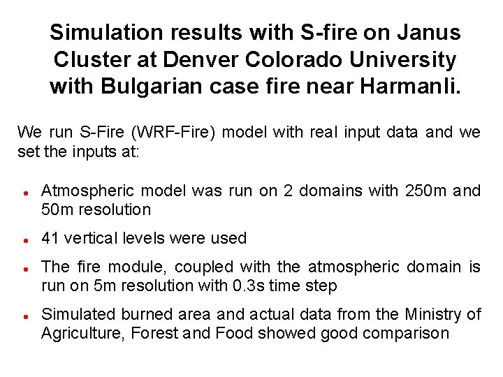
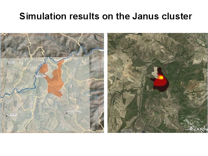
Simulation results with S-fire on Janus Cluster at Denver Colorado University with Bulgarian case fire near Harmanli. We run S-Fire (WRF-Fire) model with real input data and we set the inputs at: Atmospheric model was run on 2 domains with 250 m and 50 m resolution 41 vertical levels were used The fire module, coupled with the atmospheric domain is run on 5 m resolution with 0. 3 s time step Simulated burned area and actual data from the Ministry of Agriculture, Forest and Food showed good comparison

Simulation results on the Janus cluster

Parallel performance Cores 6 12 24 360 480 720 Real time coefficients 10. 59 9. 21 3. 91 2. 75 1. 64 0. 99 0. 61 0. 44 0. 37 0. 31 36 60 120 240 Computations were performed on the Janus cluster at the University of Colorado. The computer consists of nodes with dual Intel X 5660 processors (total 12 cores per node), connected by QDR Infini. Band The model runs as fast as real time on 120 cores and it is twice faster on 360 (real time coef. = 0. 99)

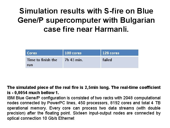
Simulation results with S-fire on Blue Gene/P supercomputer with Bulgarian case fire near Harmanli. Cores 100 cores 128 cores Time to finish the run 7 h 43 min. failed The simulated piece of the real fire is 2, 5 min long. The real-time coefficient is - 0, 0054 much bellow 1. IBM Blue Gene/P configuration is consisted of two racks with 2048 computational nodes connected by Power. PC lines, 450 processors, 8192 cores and total 4 TB operational memory. Every core can process two data streams (with double precision) after the floating point. Sixteen input-output nodes are connected by optical connection 10 Gb/s Ethernet

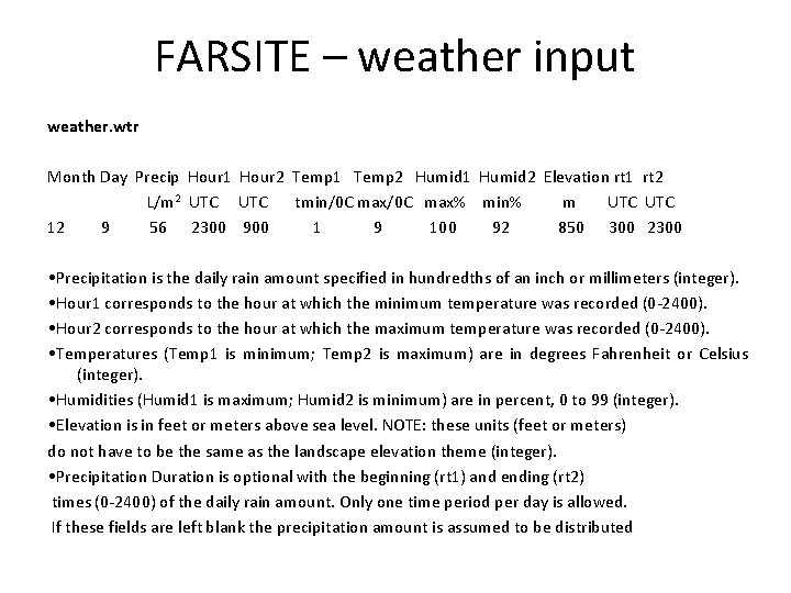
FARSITE – weather input weather. wtr Month Day Precip Hour 1 Hour 2 Temp 1 Temp 2 Humid 1 Humid 2 Elevation rt 1 rt 2 L/m 2 UTC tmin/0 C max% min% m UTC 12 9 56 2300 900 1 9 100 92 850 300 2300 • Precipitation is the daily rain amount specified in hundredths of an inch or millimeters (integer). • Hour 1 corresponds to the hour at which the minimum temperature was recorded (0 -2400). • Hour 2 corresponds to the hour at which the maximum temperature was recorded (0 -2400). • Temperatures (Temp 1 is minimum; Temp 2 is maximum) are in degrees Fahrenheit or Celsius (integer). • Humidities (Humid 1 is maximum; Humid 2 is minimum) are in percent, 0 to 99 (integer). • Elevation is in feet or meters above sea level. NOTE: these units (feet or meters) do not have to be the same as the landscape elevation theme (integer). • Precipitation Duration is optional with the beginning (rt 1) and ending (rt 2) times (0 -2400) of the daily rain amount. Only one time period per day is allowed. If these fields are left blank the precipitation amount is assumed to be distributed

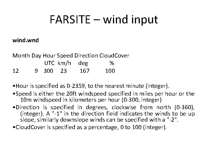
FARSITE – wind input wind. wnd Month Day Hour Speed Direction Cloud. Cover UTC km/h deg % 12 9 300 23 167 100 • Hour is specified as 0 -2359, to the nearest minute (integer). • Speed is either the 20 ft windspeed specified in miles per hour or the 10 m windspeed in kilometers per hour (0 -300, integer) • Direction is specified in degrees, clockwise from north (0 -360), (integer). A "-1" in the direction field indicates the winds to be up slope, similarly downslope winds can be specified with a "-2". • Cloud. Cover is specified as a percentage, 0 to 100 (integer).

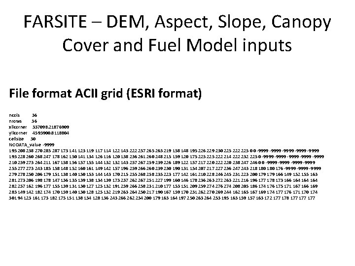
FARSITE – DEM, Aspect, Slope, Canopy Cover and Fuel Model inputs File format ACII grid (ESRI format) ncols 36 nrows 36 xllcorner 337098. 21876909 yllcorner 4593900. 8118804 cellsize 30 NODATA_value -9999 195 208 238 270 285 287 173 141 123 119 117 114 122 143 222 257 265 263 219 158 148 195 226 229 230 225 222 225 0 0 -9999 -9999 193 228 260 268 247 178 162 150 141 134 126 116 120 138 236 261 260 248 215 159 120 175 225 222 214 222 232 225 0 -9999 -9999 210 259 273 264 211 167 158 156 157 155 144 132 143 257 267 259 239 226 189 122 157 217 220 222 220 238 247 246 0 0 -9999 255 277 273 243 185 158 148 152 160 161 149 142 157 196 259 266 260 239 230 190 131 154 207 217 227 236 247 243 218 180 176 -9999 278 250 206 179 151 138 140 153 144 143 170 215 255 268 258 235 223 177 142 161 210 228 246 245 231 223 200 179 166 149 152 155 163 281 273 206 198 178 147 136 135 139 138 134 139 173 237 262 267 251 227 199 160 146 178 236 263 272 263 221 216 196 177 178 173 166 164 164 282 257 162 196 177 155 139 131 130 127 125 132 191 259 266 258 231 210 177 153 151 209 259 274 276 274 208 205 186 174 176 175 171 167 166 169 283 149 142 182 174 170 159 140 130 128 125 132 219 263 264 250 217 190 167 159 170 231 262 270 269 244 162 165 167 169 174 177 176 171 170 174 301 94 123 161 173 182 175 151 138 134 128 136 243 266 262 234 200 179 163 164 197 250 263 264 253 195 163 159 157 163 172 177 178 177 177

Zlatograd test area - Data availability 1. Digital Elevation Model for the area of Zlatograd forestry department 2. Meteorology inputs in the required formats of the FARSITE model 3. FBFMs (Fire Behavior Fuel Models) had to be developed for the area

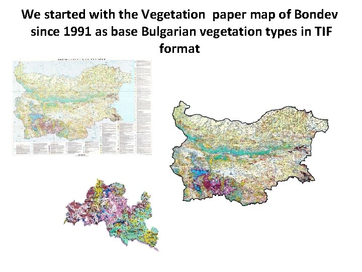
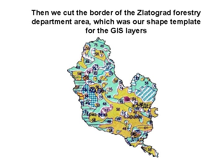
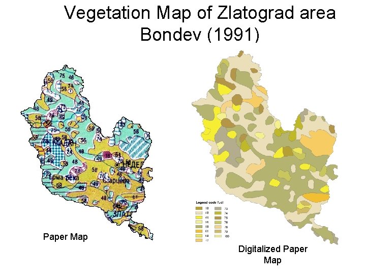
We started with the Vegetation paper map of Bondev since 1991 as base Bulgarian vegetation types in TIF format

Then we cut the border of the Zlatograd forestry department area, which was our shape template for the GIS layers

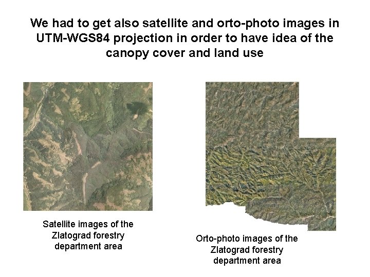
We had to get also satellite and orto-photo images in UTM-WGS 84 projection in order to have idea of the canopy cover and land use Satellite images of the Zlatograd forestry department area Orto-photo images of the Zlatograd forestry department area

Vegetation Map of Zlatograd area Bondev (1991) Paper Map Digitalized Paper Map

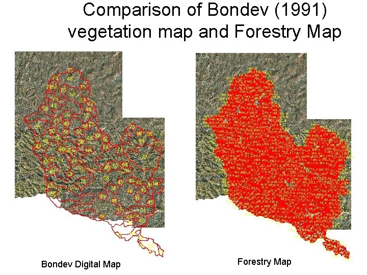
Comparison of Bondev (1991) vegetation map and Forestry Map Corine Map Bondev Digital Map Forestry Map

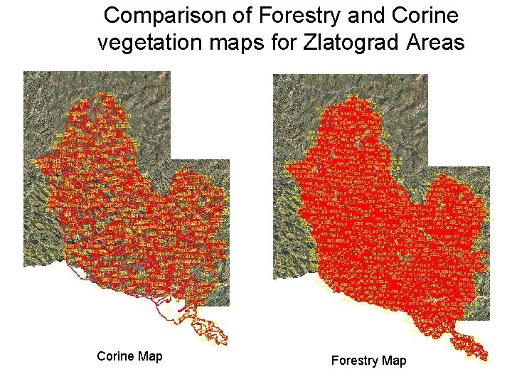
Comparison of Forestry and Corine vegetation maps for Zlatograd Areas Corine Map Forestry Map

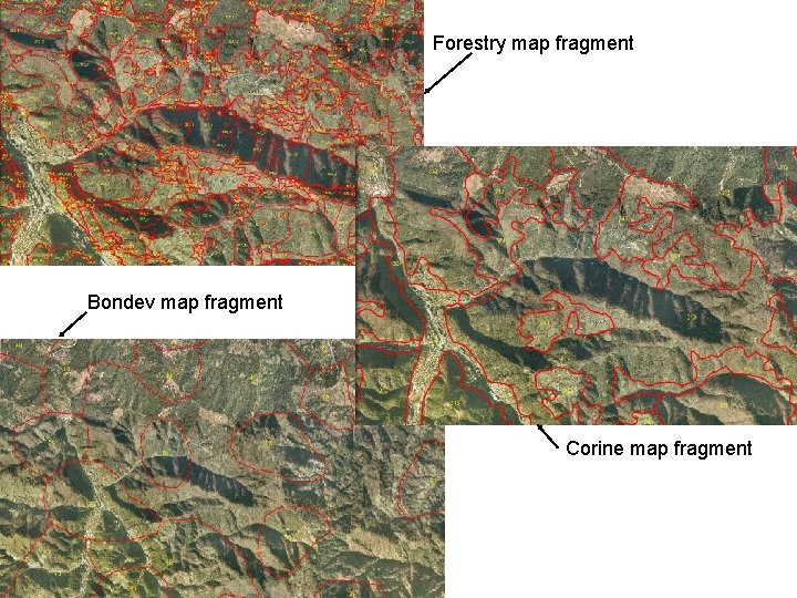
Forestry map fragment Bondev map fragment Corine map fragment

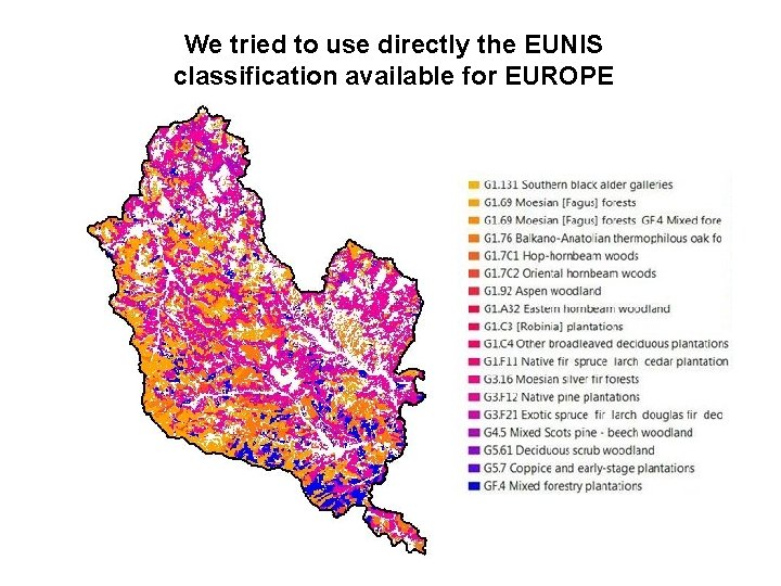
We tried to use directly the EUNIS classification available for EUROPE

FBFMs in Rothermel theory are 53 classes Anderson from 1982 with 13 classes Fire Behavior Fuel Models (FBFMs) And Scott-Burgan from 2005 with their 40 classes FBFMs

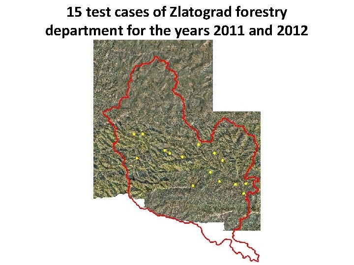
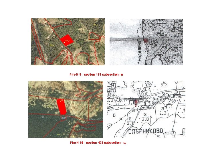
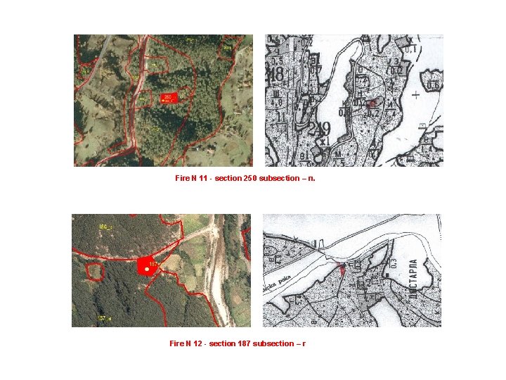
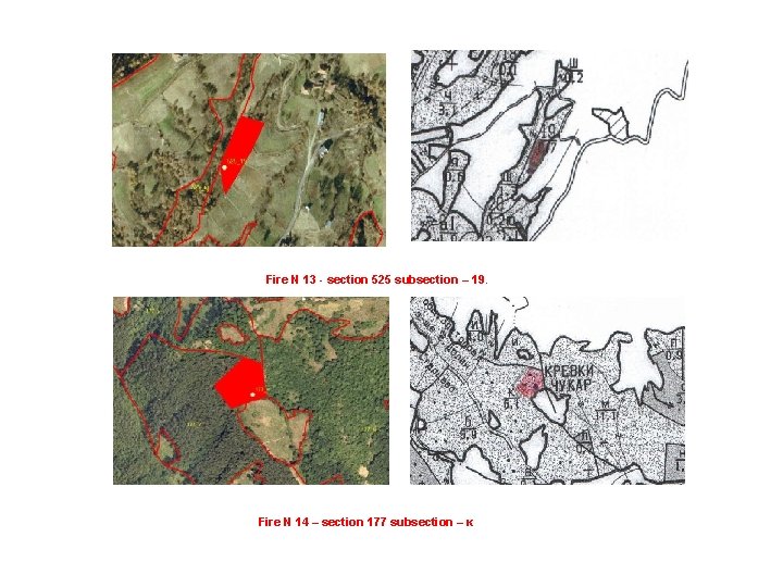
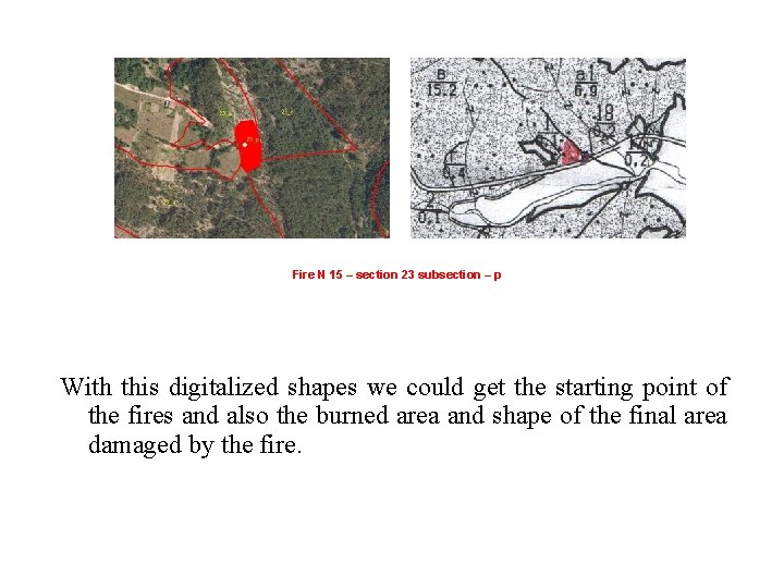
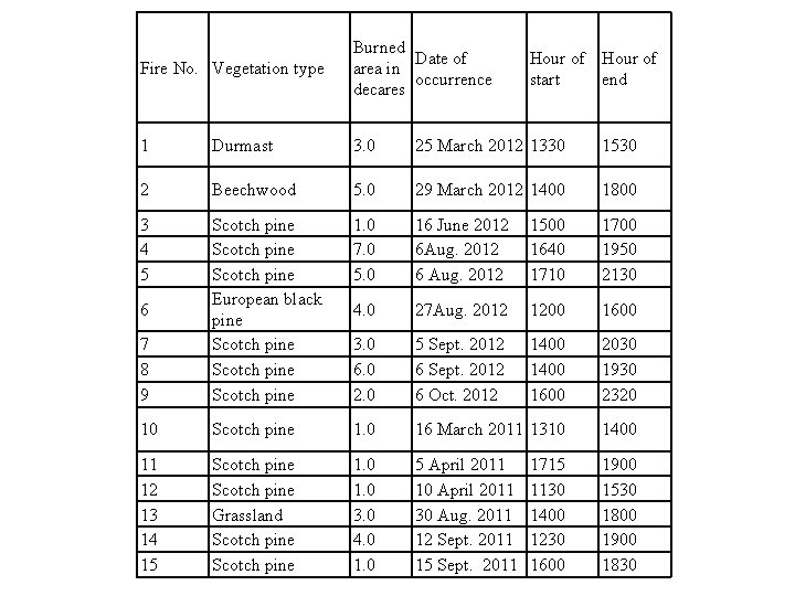
15 test cases of Zlatograd forestry department for the years 2011 and 2012

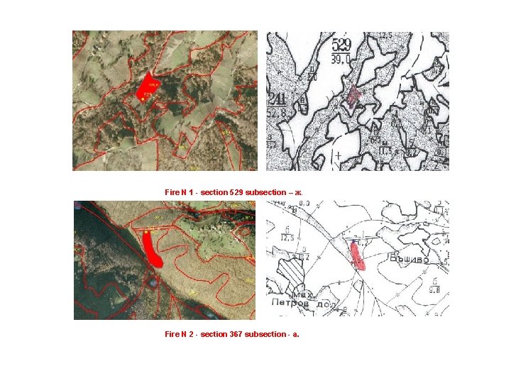
Fire N 1 - section 529 subsection – ж. Fire N 2 - section 367 subsection - а.

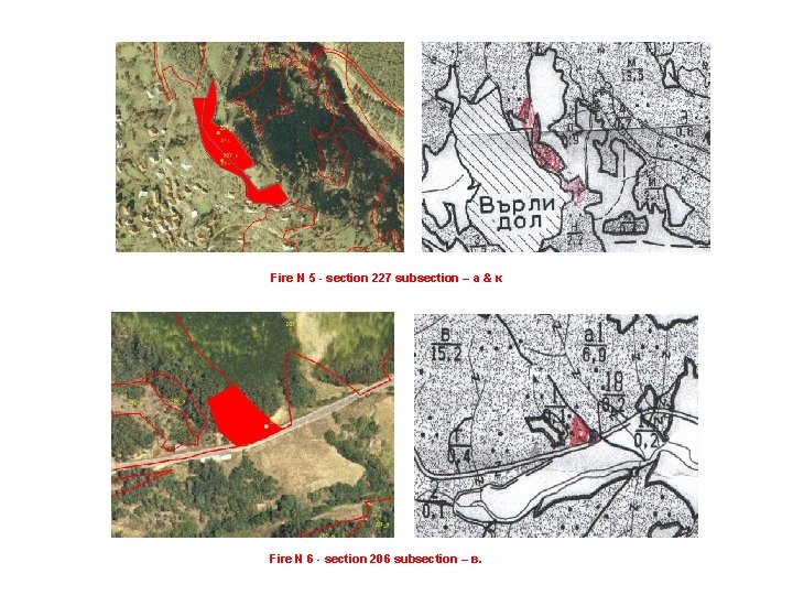
Fire N 5 - section 227 subsection – а & к Fire N 6 - section 206 subsection – в.

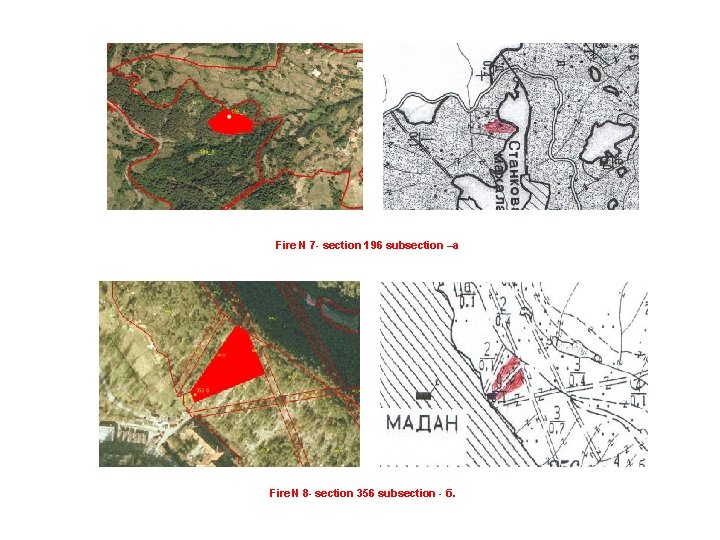
Fire N 7 - section 196 subsection –а Fire N 8 - section 356 subsection - б.

Fire N 9 - section 179 subsection– в Fire N 10 - section 423 subsection - ц.

Fire N 11 - section 250 subsection – п. Fire N 12 - section 187 subsection – г

Fire N 13 - section 525 subsection – 19. Fire N 14 – section 177 subsection – к

Fire N 15 – section 23 subsection – р With this digitalized shapes we could get the starting point of the fires and also the burned area and shape of the final area damaged by the fire.

Fire No. Vegetation type Burned Date of area in occurrence decares 1 Durmast 3. 0 25 March 2012 1330 1530 2 Beechwood 5. 0 29 March 2012 1400 1800 3 4 5 1. 0 7. 0 5. 0 16 June 2012 6 Aug. 2012 6 Aug. 2012 1500 1640 1710 1700 1950 2130 4. 0 27 Aug. 2012 1200 1600 7 8 9 Scotch pine European black pine Scotch pine 3. 0 6. 0 2. 0 5 Sept. 2012 6 Oct. 2012 1400 1600 2030 1930 2320 10 Scotch pine 1. 0 16 March 2011 1310 1400 11 12 13 14 15 Scotch pine Grassland Scotch pine 1. 0 3. 0 4. 0 1. 0 5 April 2011 10 April 2011 30 Aug. 2011 12 Sept. 2011 15 Sept. 2011 1900 1530 1800 1900 1830 6 Hour of start end 1715 1130 1400 1230 1600

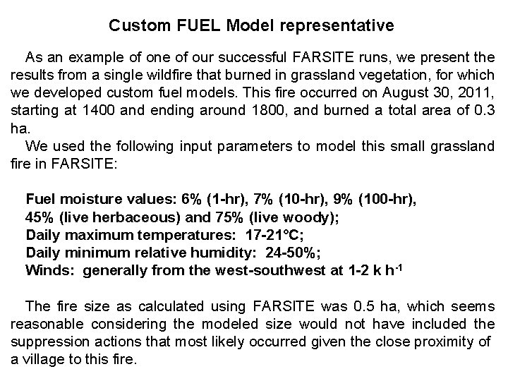
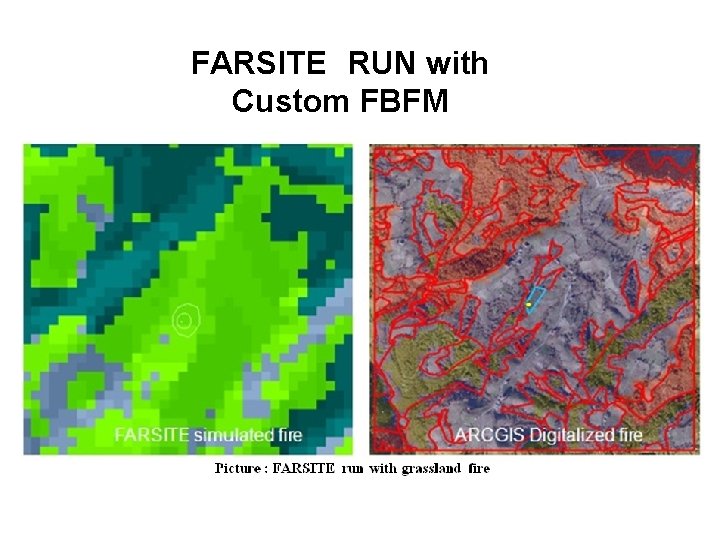
Custom FUEL Model representative As an example of one of our successful FARSITE runs, we present the results from a single wildfire that burned in grassland vegetation, for which we developed custom fuel models. This fire occurred on August 30, 2011, starting at 1400 and ending around 1800, and burned a total area of 0. 3 ha. We used the following input parameters to model this small grassland fire in FARSITE: Fuel moisture values: 6% (1 -hr), 7% (10 -hr), 9% (100 -hr), 45% (live herbaceous) and 75% (live woody); Daily maximum temperatures: 17 -21°C; Daily minimum relative humidity: 24 -50%; Winds: generally from the west-southwest at 1 -2 k h-1 The fire size as calculated using FARSITE was 0. 5 ha, which seems reasonable considering the modeled size would not have included the suppression actions that most likely occurred given the close proximity of a village to this fire.

FARSITE RUN with Custom FBFM

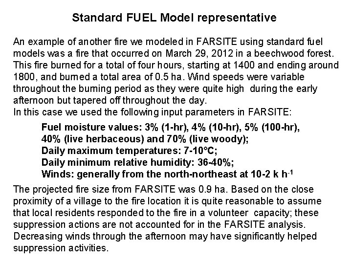
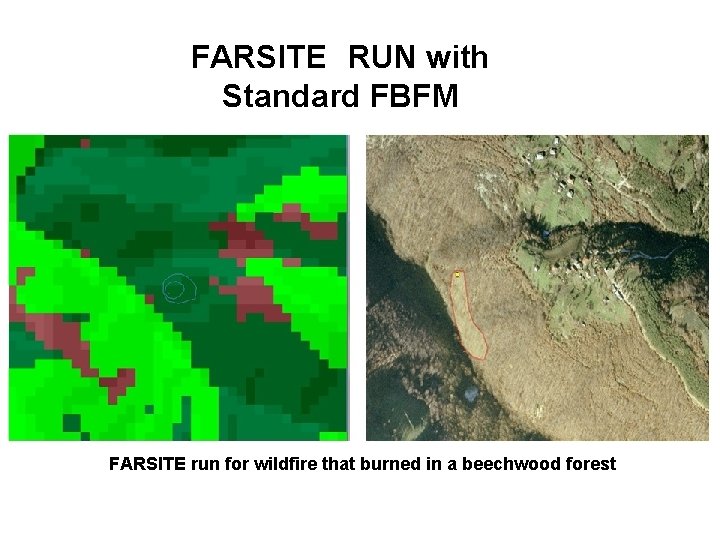
Standard FUEL Model representative An example of another fire we modeled in FARSITE using standard fuel models was a fire that occurred on March 29, 2012 in a beechwood forest. This fire burned for a total of four hours, starting at 1400 and ending around 1800, and burned a total area of 0. 5 ha. Wind speeds were variable throughout the burning period as they were quite high during the early afternoon but tapered off throughout the day. In this case we used the following input parameters in FARSITE: Fuel moisture values: 3% (1 -hr), 4% (10 -hr), 5% (100 -hr), 40% (live herbaceous) and 70% (live woody); Daily maximum temperatures: 7 -10°C; Daily minimum relative humidity: 36 -40%; Winds: generally from the north-northeast at 10 -2 k h-1 The projected fire size from FARSITE was 0. 9 ha. Based on the close proximity of a village to the fire location it is quite reasonable to assume that local residents responded to the fire in a volunteer capacity; these suppression actions are not accounted for in the FARSITE analysis. Decreasing winds through the afternoon may have significantly helped suppression activities.

FARSITE RUN with Standard FBFM FARSITE run for wildfire that burned in a beechwood forest

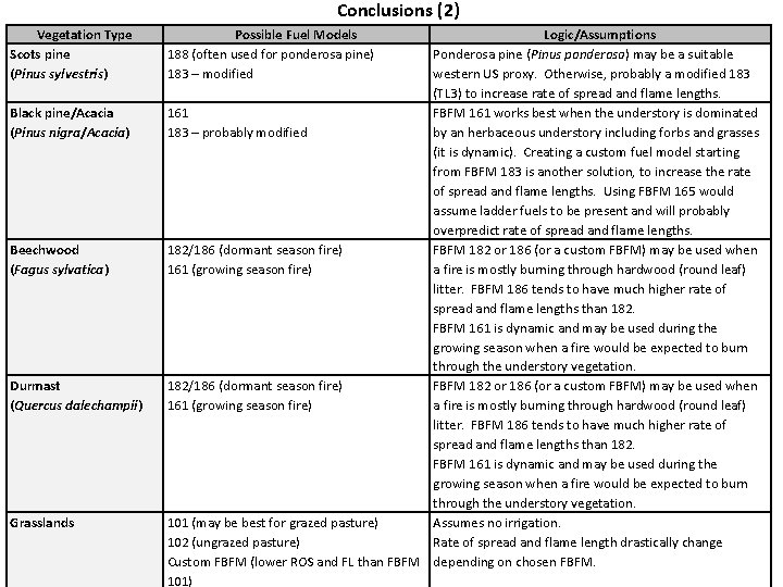
Conclusions (1) The presented work shows that from the botanical vegetation types for the test area of Zlatograd forestry department we could estimate nice approximations which in case of computer based simulations can give us reasonable output burned shapes of the wildland fire spread. Summary of this classification is given in the next table.

Conclusions (2) Vegetation Type Scots pine (Pinus sylvestris) Black pine/Acacia (Pinus nigra/Acacia) Beechwood (Fagus sylvatica) Durmast (Quercus dalechampii) Grasslands Possible Fuel Models 188 (often used for ponderosa pine) 183 – modified Logic/Assumptions Ponderosa pine (Pinus ponderosa) may be a suitable western US proxy. Otherwise, probably a modified 183 (TL 3) to increase rate of spread and flame lengths. 161 FBFM 161 works best when the understory is dominated 183 – probably modified by an herbaceous understory including forbs and grasses (it is dynamic). Creating a custom fuel model starting from FBFM 183 is another solution, to increase the rate of spread and flame lengths. Using FBFM 165 would assume ladder fuels to be present and will probably overpredict rate of spread and flame lengths. 182/186 (dormant season fire) FBFM 182 or 186 (or a custom FBFM) may be used when 161 (growing season fire) a fire is mostly burning through hardwood (round leaf) litter. FBFM 186 tends to have much higher rate of spread and flame lengths than 182. FBFM 161 is dynamic and may be used during the growing season when a fire would be expected to burn through the understory vegetation. 101 (may be best for grazed pasture) Assumes no irrigation. 102 (ungrazed pasture) Rate of spread and flame length drastically change Custom FBFM (lower ROS and FL than FBFM depending on chosen FBFM. 101)

Acknowledgements This work has been supported by the Bulgarian Academy of Sciences Program for support of young researchers No: ДФНП-95 -А 1 and by the National Science Fund of the Bulgarian Ministry of Education, Youth and Science under Grant FNI I 02/20

Thank you for your attention! Nina Dobrinkova nido@math. bas. bg