Hyperspectral Image Segmentation AZMI HAIDER LOAY MUALEM HYPERSPECTRAL

Hyperspectral Image Segmentation AZMI HAIDER LOAY MUALEM HYPERSPECTRAL IMAGING SEMINAR - PROF. HAGIT HEL-OR

Content ◦ Introduction ◦ What is segmentation? ◦ What’s the goal? ◦ Two segmentation methods: ◦ Watershed segmentation ◦ Minimum spanning forest segmentation ◦ Summary ◦ comparison

What is segmentation Dividing the image into different regions. Separating objects from background and giving them individual IDs (labels).

Why segment? Suppose we want to analyze an object in image (and not the whole image). ◦ First, we need to find its location!

Segmentation vs classification! In classification, we agree from the start on a fixed number of classes. Then we classify each pixel to a class. Pixels are connected to regions most of the time and needs to be treated with respect to neighboring pixels.

Segmentation in Hyperspectral Images Every pixel contains a detailed spectrum (>100 spectral bands) ◦ More information per pixel ◦ Dimensionality increases Advanced algorithms are required to link all channels!

Method I: Watershed segmentation Motivation: A watershed is an extent or an area of land where surface water from rain converges to a single point at a lower elevation.

Watershed transformation Input: one-band image Value of each pixel: the gradient magnitude in that pixel. Watershed lines divide the image into segments! Each segment is associated with one minimum in the image.

Gradients The gradient defines transitions between regions: ◦ it has high values on the borders between objects ◦ It has minima in the homogeneous regions. Original image gradient image in the x direction gradient image in the y direction

Flood inside borders All points inside borders are labeled to same segment!

Meyer's Flooding Algorithm One of the most common watershed algorithms. 1. A set of pixels (called markers) where the flooding shall start, are chosen. Each is given a different label.

Meyer's Flooding Algorithm 2. The neighboring pixels of each marked area are inserted into a priority queue with a priority level corresponding to the gradient magnitude of the pixel. neighboring pixels Chosen pixel

Meyer's Flooding Algorithm 3. The pixel with the lowest priority level is extracted from the priority queue. If it is labeled. Do nothing. If extracted pixel has a labeled neighbor, it is labeled with same label If it has more than one labeled neighbor (of different labels) it is watershed line! Add all it’s unlabeled neighbors to queue. 4. Redo step 3 until the priority queue is empty.

Algorithm run Given an area where numbers are the gradient magnitudes of the pixels. We start the flood from the local minimas And priority queue is empty: 3 2 2 3 1 1 0

Algorithm run Each 0 is given a different label. Labeled 0 are added to queue 00 3 2 2 3 1 1 0

Algorithm run First 0 is extracted, and all neighbors added 1110 3 2 2 3 1 1 0

Algorithm run Second 0 extracted, all neighbors added. 3111 3 2 2 3 1 1 0

Algorithm run 1 is extracted, has one neighbor with label (blue 0) It is labeled with same label. All its neighbors added to queue 32211 3 2 2 3 1 1 0

Algorithm run Another 1 is extracted, has two neighbors of different labels Labeled as W (watershed boundary) All its neighbors added to queue 33221 3 2 2 3 1 1 0

Algorithm run Same process for the last 1 Labeled as W (watershed boundary) All its neighbors added to queue 3322 3 2 2 3 1 1 0

Algorithm run Extract 2 from the queue, has one blue neighbor. Label it with same label 332 3 2 2 3 1 1 0

Algorithm run Extract second 2 from the queue, has one blue neighbor. Label it with same label 33 3 2 2 3 1 1 0

Algorithm run Extract 3 from the queue, has one blue neighbor. Label it with same label 3 3 2 2 3 1 1 0

Algorithm run Extract last 3 from the queue, has two labeled neighbors. Label as W (watershed line) 3 2 2 3 1 1 0

Algorithm run Queue is empty -> terminate. Output: segment A, Segment B, Watershed line A A A W W A B W A

Problem: over segmentation Every single local minimum of the gradient leads to one region. Some local minimas are formed due to noise, minor fluctuations in brightness, etc. . !

Solutions I: thresholding All minimas under a certain threshold are not accepted as minima. This is done before the flooding.

Solution II: smooth image before gradient A) original image B) gradient of image C) watershed on b D) watershed on smoothed image

Solution III: controlled-markers User markers to specify which are the regions of interest. Internal markers: specifies objects. External markers: specifies background. Regions with no internal markers can be merged into one region.

Choosing the marker: ◦ Automatic: Another algorithm ◦ Manual: User selection.

Problem: sensitive edges At some point in the algorithm we chose to extract 3. Which 3? Suppose we extracted the other 3. 33 3 2 2 3 1 1 0

Problem: sensitive edges It has one neighbor of label. 3 3 2 2 3 1 1 0

Problem: sensitive edges The last 3 will be watershed line. 3 2 2 3 1 1 0

Problem: sensitive edges The edge is changed. W A A A B W A W W A B W A

Solution: use edge detectors to strengthen watershed lines Combine watershed lines with edge detector results. 1 0 0 3 2 2 0 1 0 3 1 1 0 0 1 0

Solution: use edge detectors to strengthen watershed lines The 4 will be at the end of the priority queue, forcing the 3 to be labeled before. 4 2 2 3 2 1 0 2 0

Watershed segmentation in hyperspectral images Input: Multi-band image

Feature extraction stage The aim of this step is to obtain either a one-band image or a multi-band image which would contain enough information to distinguish between spatial structures in the image. It’s done with: ◦ Principal Component Analysis (PCA) ◦ Maximum Noise Fraction (MNF) ◦ Independent Component Analysis (ICA)

Gradient stage Input: the output of feature extraction stage If Input is one-band image => Gradient is straightforward. If not, we need to proceed with a multi-band image: ◦ Vectorial gradient ◦ Multidimensional gradient ◦ combine watershed segmentation maps a posteriori

Vectorial gradient: metricbased gradient

Vectorial gradient: Color Morphological Gradient

Multidimensional gradient method

One gradient image output

Watershed on output gradient image Given one gradient image that combines gradient information from all gradient images of all B bands. We perform watershed segmentation on it.

Multidimensional segmentation maps For each gradient image in each band, we perform watershed segmentation: ◦ Output: binary watershed lines image. => B binary maps containing watershed lines.

Combine all gradients and Watershed / Watershed all gradients and combine? When summing the watershed lines, we do not have information about regions anymore! but only about edges. Suppose B-1 bands had the previous image. One band had this image => (no matter how large the gradient was this segment will disappear when thresholding) Only one band has this segment

Minimum Spanning Forest Segmentation

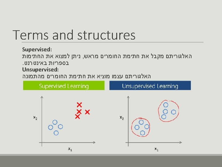
Terms and structures

Terms and structures MSF : Minimum Spanning Forest

Terms and structures Oversegmentation : One region is detected as several ones of the image. Undersegmentation : Several regions are detected as one.

Input

Output’s The algorithm contains 4 steps. After step will provide the following output’s : Scale of colors to represent probabilities 0%-bottom 100% - top 1) Pixelwise classification map 2) Probability map Pixelwise classification map Probability map

Output’s After step 4 The Algorithm provides the following output - Classification map obtained using the SAM dissimilarity measure and including a majority voting step. Classification map using SAM and majority voting

The Algorithm has 4 steps and it’s based on the construction of a MSF from region markers , which are defined automatically from classification results. After that , the Algorithm construct a MSF , and each tree in the MSF grown from a marker forms a region in the segmentation map. Last , the classification map is refined using the pixelwise classification results and the majority voting.

The 4 steps of the Algorithm: A. Pixelwise classification B. Selection of the most Reliable classified Pixels C. Construction of a MSF D. Majority Voting Within Connected Components

Scheme

A. Pairwise classification The first step consists in performing a probabilistic Pixelwise classification of the hyperspectral image. We propose to use a Support vector machine (SVM) classifier Classification consists of assigning each pixel to one of the K classes of interest.

The outputs of this step are the following: 1) Classification map, containing class labels for each pixel Pixelwise classification map 2) Probability map, containing probability estimates for Scale of colors to represent probabilities 0%-bottom 100% - top Each pixel to belong to the assigned class. Probability map

Probabilities to each class for pixel x

A. Pairwise classification For further information please check [3]

A. Pairwise classification

A. Pairwise classification üThis problem has a unique solution and can be solved by a simple linear system. üFinally, a probability map is constructed by assigning to each pixel the maximum probability estimate Scale of colors to represent probabilities 0%-bottom 100% - top Probability map

B. Selection of the Most Reliable Classified Pixels The aim of this step is to choose the most reliable classified pixels in order to define suitable markers.

B. Selection of the Most Reliable Classified Pixels • Marker selection by thresholding the probability map. • If the probability of the considered pixel belonging to the assigned k is higher than a given threshold – the pixel is selected to join the markers.

B. Selection of the Most Reliable Classified Pixels §In the resulting map of markers, each marker pixel is associated with the class defined by the pixelwise classifier §The marker pixels form connected components in the map of markers so that each connected component represents one marker.

Advantage and Disadvantage ü Advantage : Simplicity ü Easy to select markers ü Simple calculations × Disadvantage : × As many markers as the desired number of regions. × Undersegmentation

Disadvantage’s

Solution To mitigate this problem, we propose the following method of marker selection 1) Perform a connected-component labeling of the pixelwise classification map. For this purpose, a classical connected component algorithm using the union-find data structure.

Solution 2) Analyze each connected region as follows. • If a region is large enough, it should contain a marker, which is determined as P% of the pixels within the connected component with the highest probability estimates. • If a region is small, it should lead to a marker only if it is very reliable; a potential marker is formed by pixels with probability estimates higher than a defined threshold.

Example of marker selection Each connected spatial region from the classification map is analyzed if it corresponds most probably to the spatial structure or if it is rather a classification noise

Example of marker selection § If the size of the component is large enough to consider it as a relevant region, the most reliable pixels within this region are selected as its marker. §If a component contains only a few pixels, it is investigated if these pixels were classified to a particular class with a high probability. ü If this is the case, the considered connected component represents a small spatial structure. Thus, a marker associated with this region should be defined. × Otherwise, the component is the consequence of classification noise, and we tend to eliminate it.

Parameters & markers selection procedure §A parameter M defining if a region is considered as being large or small. § A parameter P, defining the percentage of pixels within the large region to be used as markers. §The last parameter S, which is a threshold of probability estimates defining potential markers for a small region.

The Procedure

The Procedure

The Procedure

C. Construction of an MSF : minimum spanning forst. The previous two steps result in a map of markers defining regions of interest in the image. The next step consists in the grouping of all the image pixels into an MSF, where each tree is rooted on a classificationderived marker.

C. Construction of an MSF

C. Construction of an MSF

Different dissimilarity measure

Different dissimilarity measure

Different dissimilarity measure

Final MSF

Final MSF

Result §Each tree in the MSF forms a region in the segmentation map (by mapping the resulting graph onto an image). §The proposed procedure of the construction of an MSF from region markers is a region growing method

Result

D. Majority Voting Within Connected Components Although the most reliable classified pixels are selected as markers, it may happen that a marker is classified to the wrong class. In this case, all the pixels within the region grown from this marker risk to be wrongly classified.

D. Majority Voting Within Connected Components

D. Majority Voting Within Connected Components When performing the last majority voting step, the use of the four-neighborhood connectivity results in a larger or the same number of connected components as the use of the eight-neighborhood connectivity that was used for the construction of an MSF. ҂ Therefore , the possible under-segmentation can be corrected in this step. ҂One region from a segmentation map can be split into two connected regions (when using four-neighborhood) ҂These two regions can be assigned to two different classes by the majority voting step

Experimental Results

Experimental Results A pixelwise classification on the 200 -band Indiana image was performed, using the multiclass one versus one SVM classifier with the Gaussian radial basis function (RBF) kernel.

Experimental Results

Experimental Results

Experimental Results

Experimental Results

Comparison Watershed MSF Not efficient speed Accepted speed In many cases the image may over segment Almost no over segmentation Segment borders not accurate

References 1. Segmentation and classification of hyperspectral images using watershed transformation Yuliya Tarabalka, Jocelyn Chanussot, Jon Atli 2. 3. 4. Benediktsson. Segmentation and Classification of Hyperspectral Images Using Minimum Spanning Forest Grown From Automatically Selected Markers Yuliya Tarabalka, Jocelyn Chanussot, and Jón Atli Benediktsson IEEE Transactions on System Man and Cybernetics, Vol 40(5), 2010 A note on Platt’s probabilistic outputs for support vector machines, H. -T. Lin , C. -J. Lin , and R. C. Weng , Dept. Comput. Sci. , Nat. Univ. , Taipei, Taiwan, 2003 J. Platt, “Probabilistic outputs for support vector machine and comparison to regularized likelihood methods, ” in Advances in Large Margin Classifiers , A. Smola , P. Bartlett , B. Scholkopf and D. Schuurmans, Eds. Cambridge , MA: MIT Press, 200 .

Thank you