Image segmentation 1 Image Segmentation s In computer

- Slides: 1

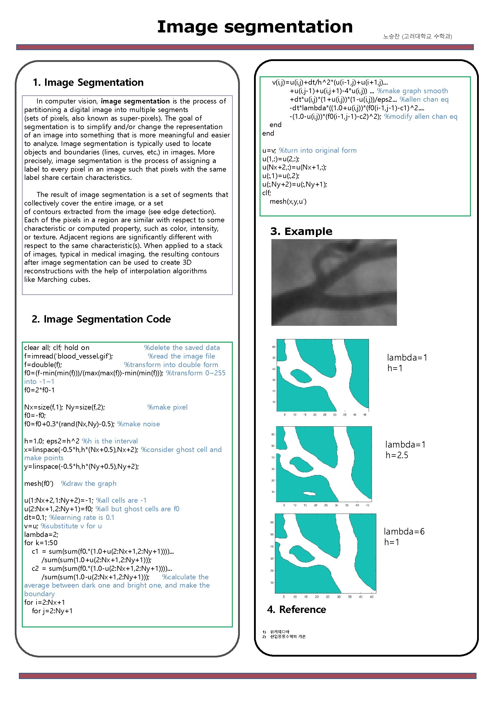
Image segmentation 1. Image Segmentation s In computer vision, image segmentation is the process of partitioning a digital image into multiple segments (sets of pixels, also known as super-pixels). The goal of segmentation is to simplify and/or change the representation of an image into something that is more meaningful and easier to analyze. Image segmentation is typically used to locate objects and boundaries (lines, curves, etc. ) in images. More precisely, image segmentation is the process of assigning a label to every pixel in an image such that pixels with the same label share certain characteristics. The result of image segmentation is a set of segments that collectively cover the entire image, or a set of contours extracted from the image (see edge detection). Each of the pixels in a region are similar with respect to some characteristic or computed property, such as color, intensity, or texture. Adjacent regions are significantly different with respect to the same characteristic(s). When applied to a stack of images, typical in medical imaging, the resulting contours after image segmentation can be used to create 3 D reconstructions with the help of interpolation algorithms like Marching cubes. 노승찬 (고려대학교 수학과) v(i, j)=u(i, j)+dt/h^2*(u(i-1, j)+u(i+1, j). . . +u(i, j-1)+u(i, j+1)-4*u(i, j)). . . %make graph smooth +dt*u(i, j)*(1+u(i, j))*(1 -u(i, j))/eps 2. . . %allen chan eq -dt*lambda*((1. 0+u(i, j))*(f 0(i-1, j-1)-c 1)^2. . -(1. 0 -u(i, j))*(f 0(i-1, j-1)-c 2)^2); %modify allen chan eq end u=v; %turn into original form u(1, : )=u(2, : ); u(Nx+2, : )=u(Nx+1, : ); u(: , 1)=u(: , 2); u(: , Ny+2)=u(: , Ny+1); clf; mesh(x, y, u') 3. Example 2. Image Segmentation Code clear all; clf; hold on %delete the saved data f=imread('blood_vessel. gif’); %read the image file f=double(f); %transform into double form f 0=(f-min(f)))/(max(f))-min(f))); %transform 0~255 into -1~1 f 0=2*f 0 -1 lambda=1 h=1 Nx=size(f, 1); Ny=size(f, 2); %make pixel f 0=-f 0; f 0=f 0+0. 3*(rand(Nx, Ny)-0. 5); %make noise h=1. 0; eps 2=h^2 %h is the interval x=linspace(-0. 5*h, h*(Nx+0. 5), Nx+2); %consider ghost cell and make points y=linspace(-0. 5*h, h*(Ny+0. 5), Ny+2); lambda=1 h=2. 5 mesh(f 0’) %draw the graph u(1: Nx+2, 1: Ny+2)=-1; %all cells are -1 u(2: Nx+1, 2: Ny+1)=f 0; %all but ghost cells are f 0 dt=0. 1; %learning rate is 0. 1 v=u; %substitute v for u lambda=2; for k=1: 50 c 1 = sum(f 0. *(1. 0+u(2: Nx+1, 2: Ny+1)))). . . /sum(1. 0+u(2: Nx+1, 2: Ny+1))); c 2 = sum(f 0. *(1. 0 -u(2: Nx+1, 2: Ny+1)))). . . /sum(1. 0 -u(2: Nx+1, 2: Ny+1))); %calculate the average between dark one and bright one, and make the boundary for i=2: Nx+1 for j=2: Ny+1 lambda=6 h=1 4. Reference 1) 2) 위키피디아 산업응용수학의 기본