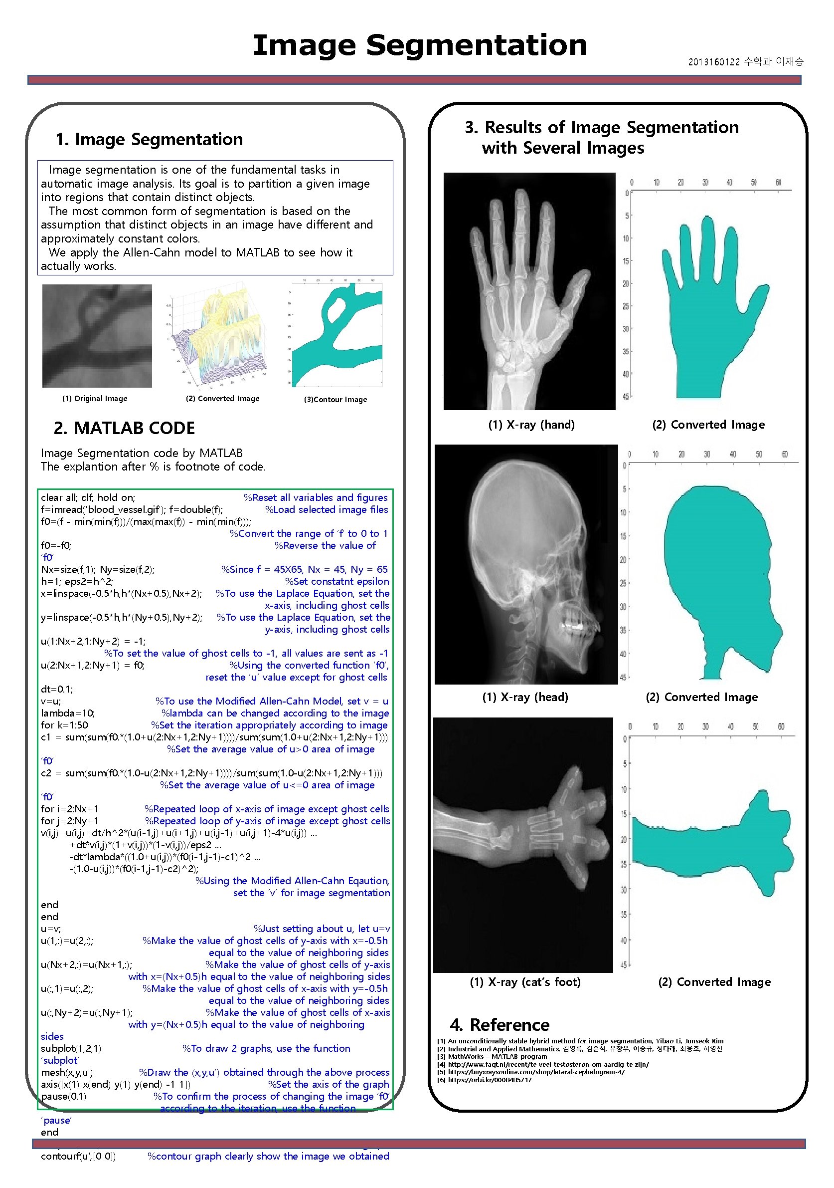
Image Segmentation 2013160122 3 Results of Image Segmentation

Image Segmentation 2013160122 수학과 이재승 3. Results of Image Segmentation with Several Images 1. Image Segmentation s Image segmentation is one of the fundamental tasks in automatic image analysis. Its goal is to partition a given image into regions that contain distinct objects. The most common form of segmentation is based on the assumption that distinct objects in an image have different and approximately constant colors. We apply the Allen-Cahn model to MATLAB to see how it actually works. (1) Original Image (2) Converted Image (3)Contour Image 2. MATLAB CODE (1) X-ray (hand) (2) Converted Image Segmentation code by MATLAB The explantion after % is footnote of code. clear all; clf; hold on; %Reset all variables and figures f=imread('blood_vessel. gif'); f=double(f); %Load selected image files f 0=(f - min(f)))/(max(f)) - min(f))); %Convert the range of ‘f’ to 0 to 1 f 0=-f 0; %Reverse the value of ‘f 0’ Nx=size(f, 1); Ny=size(f, 2); %Since f = 45 X 65, Nx = 45, Ny = 65 h=1; eps 2=h^2; %Set constatnt epsilon x=linspace(-0. 5*h, h*(Nx+0. 5), Nx+2); %To use the Laplace Equation, set the x-axis, including ghost cells y=linspace(-0. 5*h, h*(Ny+0. 5), Ny+2); %To use the Laplace Equation, set the y-axis, including ghost cells u(1: Nx+2, 1: Ny+2) = -1; %To set the value of ghost cells to -1, all values are sent as -1 u(2: Nx+1, 2: Ny+1) = f 0; %Using the converted function ‘f 0’, reset the ‘u’ value except for ghost cells dt=0. 1; v=u; %To use the Modified Allen-Cahn Model, set v = u lambda=10; %lambda can be changed according to the image for k=1: 50 %Set the iteration appropriately according to image c 1 = sum(f 0. *(1. 0+u(2: Nx+1, 2: Ny+1))))/sum(1. 0+u(2: Nx+1, 2: Ny+1))) %Set the average value of u>0 area of image ‘f 0’ c 2 = sum(f 0. *(1. 0 -u(2: Nx+1, 2: Ny+1))))/sum(1. 0 -u(2: Nx+1, 2: Ny+1))) %Set the average value of u<=0 area of image ‘f 0’ for i=2: Nx+1 %Repeated loop of x-axis of image except ghost cells for j=2: Ny+1 %Repeated loop of y-axis of image except ghost cells v(i, j)=u(i, j)+dt/h^2*(u(i-1, j)+u(i+1, j)+u(i, j-1)+u(i, j+1)-4*u(i, j)). . . +dt*v(i, j)*(1+v(i, j))*(1 -v(i, j))/eps 2. . . -dt*lambda*((1. 0+u(i, j))*(f 0(i-1, j-1)-c 1)^2. . . -(1. 0 -u(i, j))*(f 0(i-1, j-1)-c 2)^2); %Using the Modified Allen-Cahn Eqaution, set the ‘v’ for image segmentation end u=v; %Just setting about u, let u=v u(1, : )=u(2, : ); %Make the value of ghost cells of y-axis with x=-0. 5 h equal to the value of neighboring sides u(Nx+2, : )=u(Nx+1, : ); %Make the value of ghost cells of y-axis with x=(Nx+0. 5)h equal to the value of neighboring sides u(: , 1)=u(: , 2); %Make the value of ghost cells of x-axis with y=-0. 5 h equal to the value of neighboring sides u(: , Ny+2)=u(: , Ny+1); %Make the value of ghost cells of x-axis with y=(Nx+0. 5)h equal to the value of neighboring sides subplot(1, 2, 1) %To draw 2 graphs, use the function ‘subplot’ mesh(x, y, u') %Draw the (x, y, u’) obtained through the above process axis([x(1) x(end) y(1) y(end) -1 1]) %Set the axis of the graph pause(0. 1) %To confirm the process of changing the image ‘f 0’ according to the iteration, use the function ‘pause’ end subplot(1, 2, 2) %Draw the second graph contourf(u', [0 0]) %contour graph clearly show the image we obtained (1) X-ray (head) (1) X-ray (cat’s foot) (2) Converted Image 4. Reference [1] [2] [3] [4] [5] [6] An unconditionally stable hybrid method for image segmentation, Yibao Li, Junseok Kim Industrial and Applied Mathematics, 김영록, 김준석, 유창우, 이승규, 정다래, 최용호, 허영진 Math. Works – MATLAB program http: //www. faqt. nl/recent/te-veel-testosteron-om-aardig-te-zijn/ https: //buyxraysonline. com/shop/lateral-cephalogram-4/ https: //orbi. kr/0008485717