CNN architectures AZMI HAIDER MUHAMMAD SALAMAH data augmentation

CNN architectures AZMI HAIDER MUHAMMAD SALAMAH

- data augmentation Topics of the day - transfer learning - common architectures

Data augmentation • Regularization helps to prevent overfitting • Overfitting results from insufficient amount of training data We can fix this by: • Increasing the training data synthetically

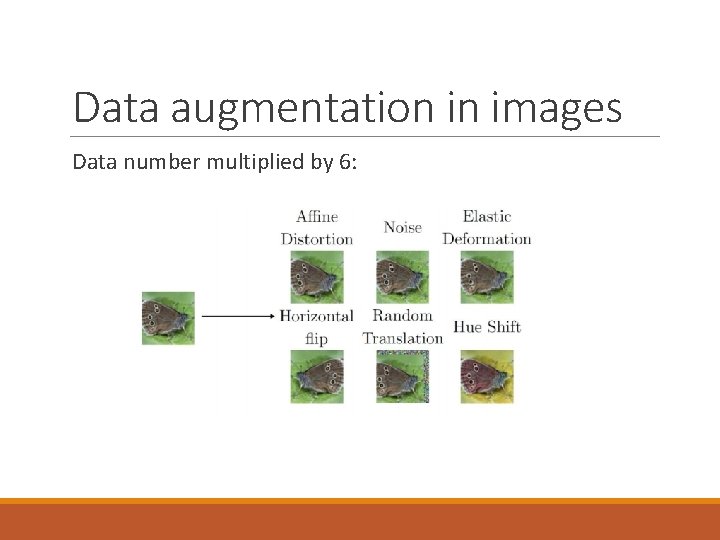
Data augmentation in images Data number multiplied by 6:

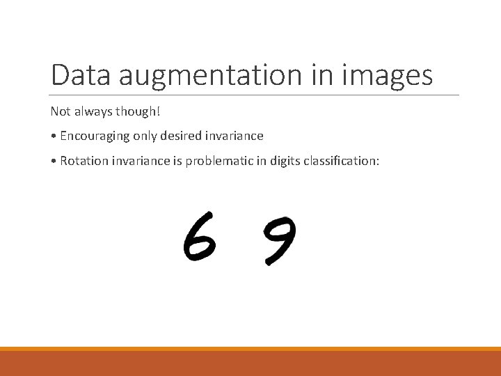
Data augmentation in images Not always though! • Encouraging only desired invariance • Rotation invariance is problematic in digits classification:

Data augmentation by noise injection • Adding random noise to inputs • Applying noise to the hidden units ◦ magnitude of the noise should be carefully tuned

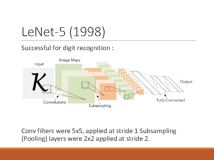
Le. Net-5 (1998) Successful for digit recognition : Conv filters were 5 x 5, applied at stride 1 Subsampling (Pooling) layers were 2 x 2 applied at stride 2.

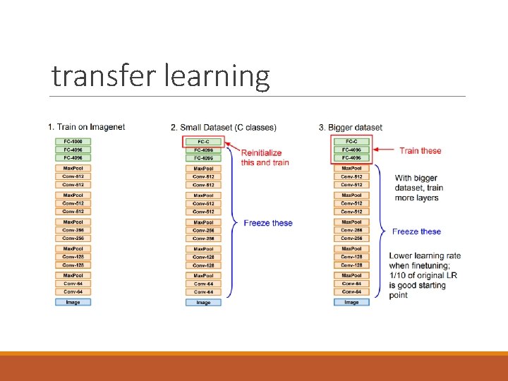
transfer learning Problem: CNN needs a huge amount of Data to be trained. Solutions: 1. Regularization 2. Transfer learning

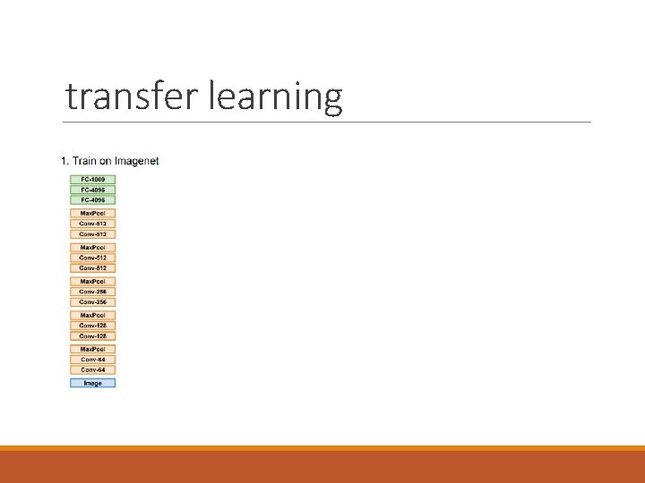
transfer learning

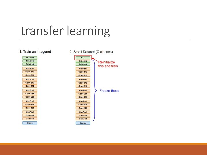
transfer learning

transfer learning

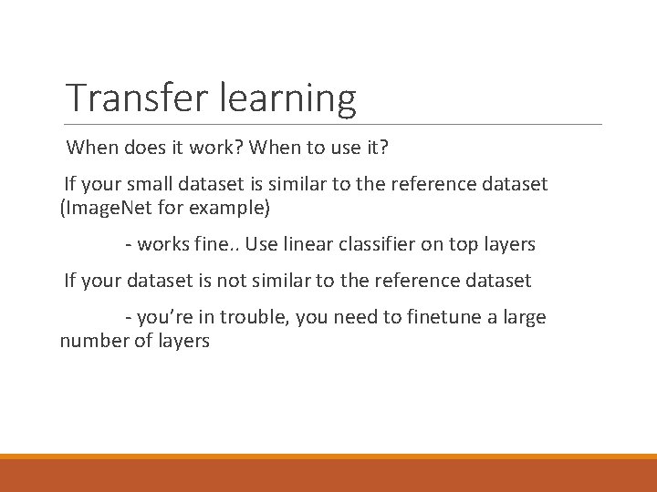
Transfer learning When does it work? When to use it? If your small dataset is similar to the reference dataset (Image. Net for example) - works fine. . Use linear classifier on top layers If your dataset is not similar to the reference dataset - you’re in trouble, you need to finetune a large number of layers

Today’s common architectures - Alex. Net - VGG - Google. Net - Res. Net

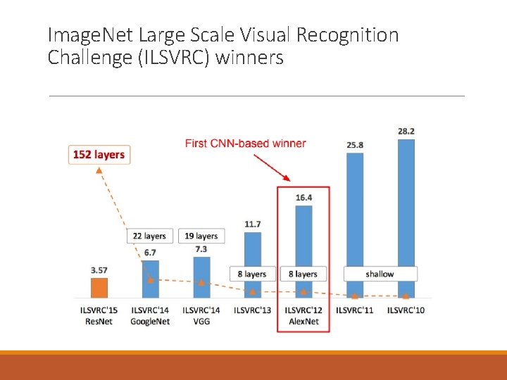
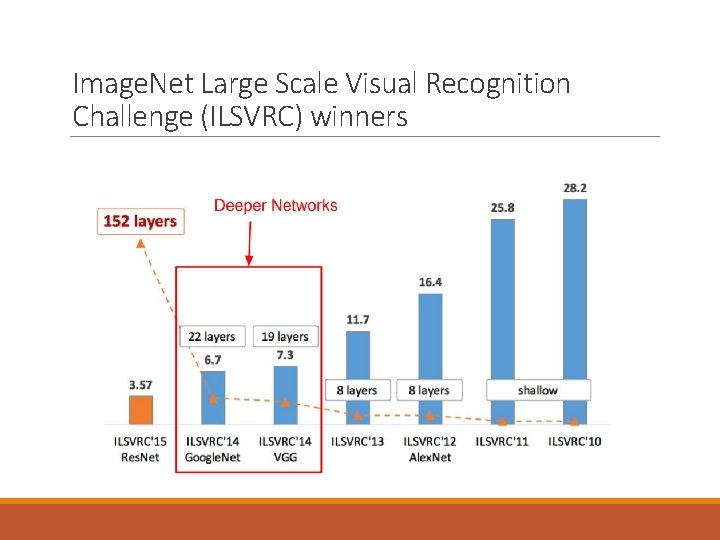
Image. Net Large Scale Visual Recognition Challenge (ILSVRC) winners

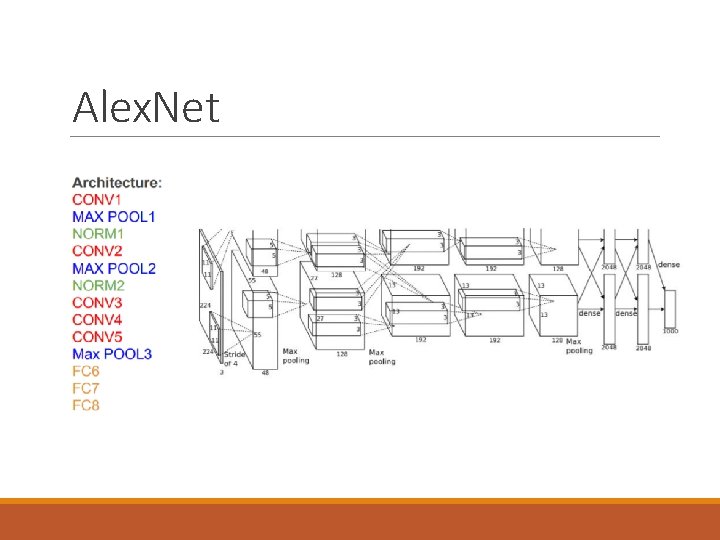
Alex. Net

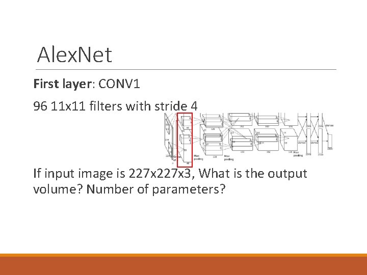
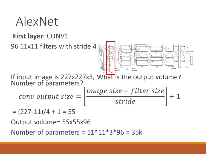
Alex. Net First layer: CONV 1 96 11 x 11 filters with stride 4 If input image is 227 x 3, What is the output volume? Number of parameters?

Alex. Net

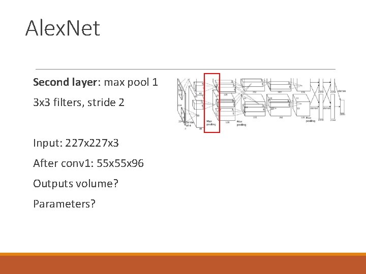
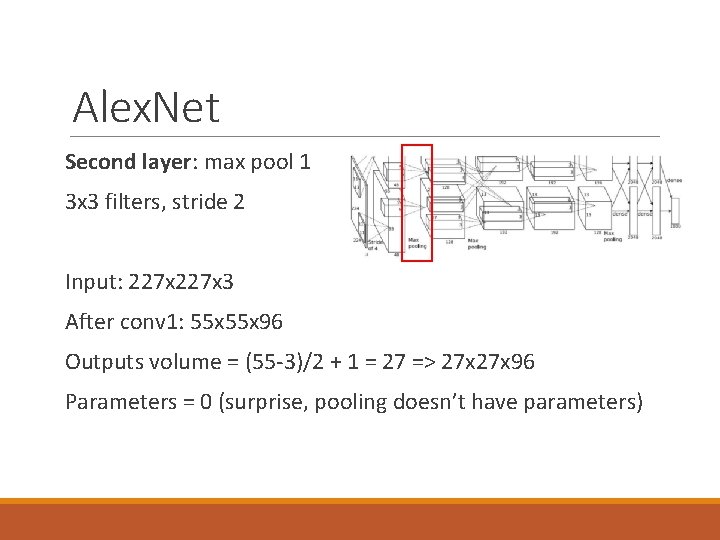
Alex. Net Second layer: max pool 1 3 x 3 filters, stride 2 Input: 227 x 3 After conv 1: 55 x 96 Outputs volume? Parameters?

Alex. Net Second layer: max pool 1 3 x 3 filters, stride 2 Input: 227 x 3 After conv 1: 55 x 96 Outputs volume = (55 -3)/2 + 1 = 27 => 27 x 96 Parameters = 0 (surprise, pooling doesn’t have parameters)

Alex. Net architecture [227 x 3] INPUT [55 x 96] CONV 1: 96 11 x 11 filters at stride 4, pad 0 [27 x 96] MAX POOL 1: 3 x 3 filters at stride 2 [27 x 96] NORM 1: Normalization layer [27 x 256] CONV 2: 256 5 x 5 filters at stride 1, pad 2 [13 x 256] MAX POOL 2: 3 x 3 filters at stride 2 [13 x 256] NORM 2: Normalization layer [13 x 384] CONV 3: 384 3 x 3 filters at stride 1, pad 1 [13 x 384] CONV 4: 384 3 x 3 filters at stride 1, pad 1 [13 x 256] CONV 5: 256 3 x 3 filters at stride 1, pad 1 [6 x 6 x 256] MAX POOL 3: 3 x 3 filters at stride 2 [4096] FC 6: 4096 neurons [4096] FC 7: 4096 neurons [1000] FC 8: 1000 neurons (class scores)

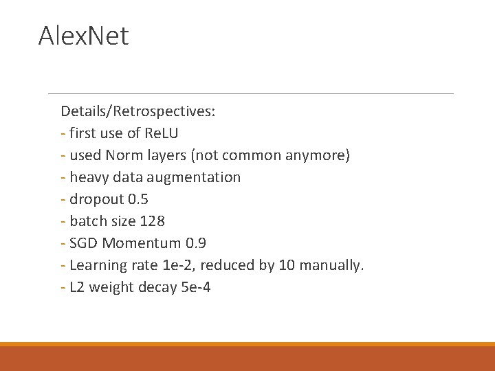
Alex. Net Details/Retrospectives: - first use of Re. LU - used Norm layers (not common anymore) - heavy data augmentation - dropout 0. 5 - batch size 128 - SGD Momentum 0. 9 - Learning rate 1 e-2, reduced by 10 manually. - L 2 weight decay 5 e-4

Image. Net Large Scale Visual Recognition Challenge (ILSVRC) winners

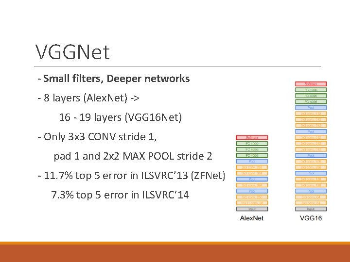
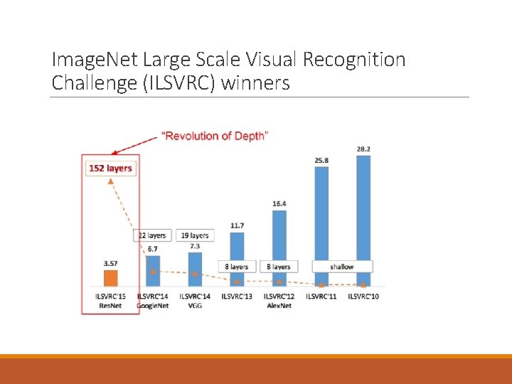
VGGNet - Small filters, Deeper networks - 8 layers (Alex. Net) -> 16 - 19 layers (VGG 16 Net) - Only 3 x 3 CONV stride 1, pad 1 and 2 x 2 MAX POOL stride 2 - 11. 7% top 5 error in ILSVRC’ 13 (ZFNet) -> 7. 3% top 5 error in ILSVRC’ 14

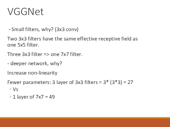
VGGNet - Small filters, why? (3 x 3 conv) Two 3 x 3 filters have the same effective receptive field as one 5 x 5 filter. Three 3 x 3 filter => one 7 x 7 filter. - deeper network, why? Increase non-linearity Fewer parameters: 3 layer of 3 x 3 filters = 3* (3*3) = 27 ◦ Vs ◦ 1 layer of 7 x 7 = 49

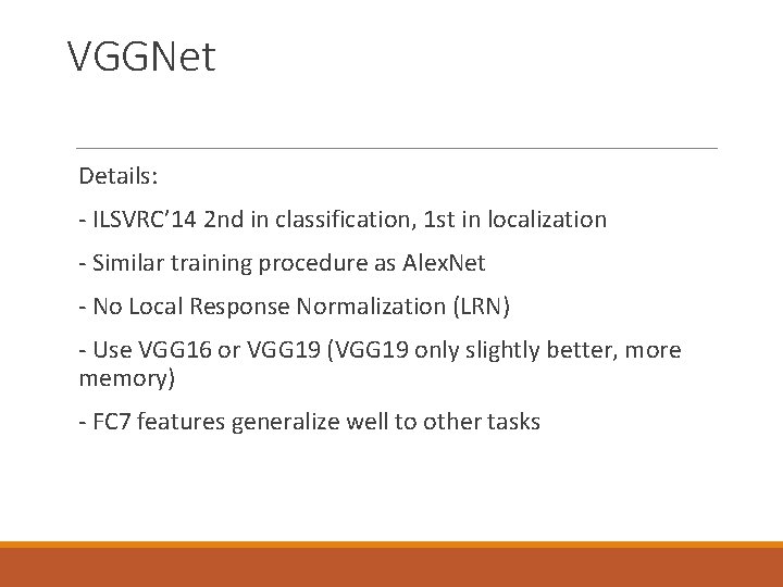
VGGNet Details: - ILSVRC’ 14 2 nd in classification, 1 st in localization - Similar training procedure as Alex. Net - No Local Response Normalization (LRN) - Use VGG 16 or VGG 19 (VGG 19 only slightly better, more memory) - FC 7 features generalize well to other tasks

Image. Net Large Scale Visual Recognition Challenge (ILSVRC) winners

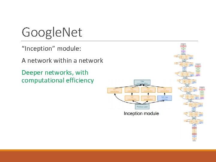
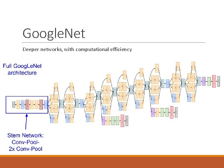
Google. Net “Inception” module: A network within a network Deeper networks, with computational efficiency

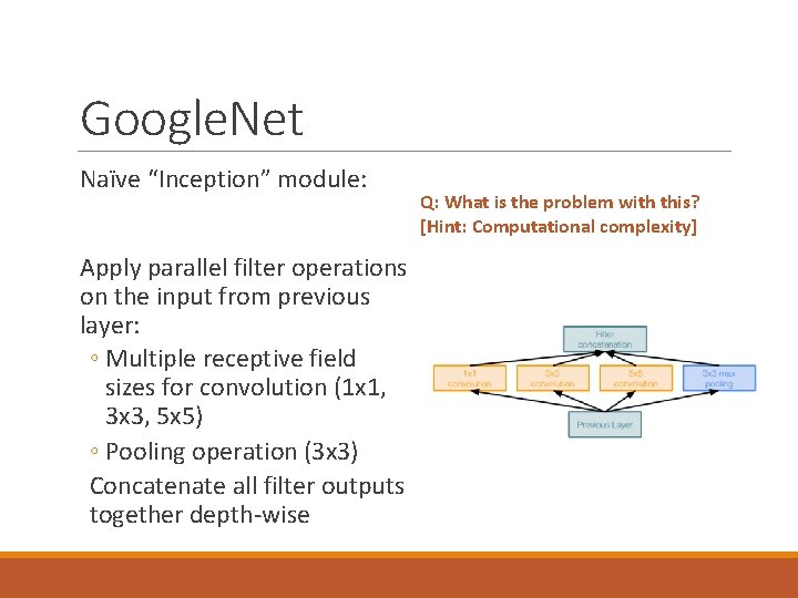
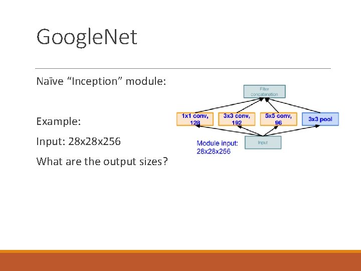
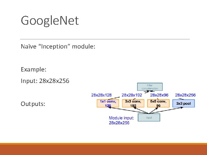
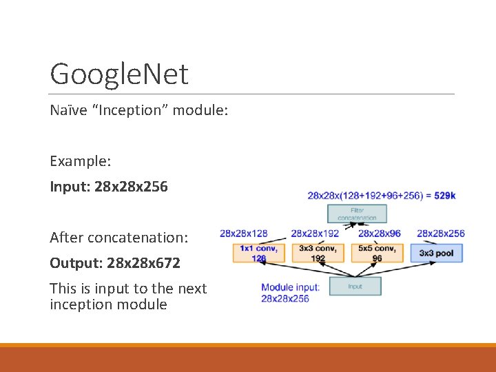
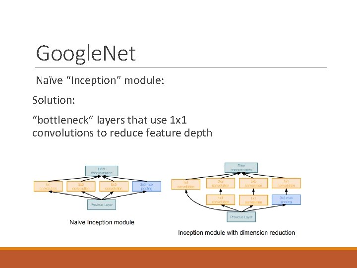
Google. Net Naïve “Inception” module: Apply parallel filter operations on the input from previous layer: ◦ Multiple receptive field sizes for convolution (1 x 1, 3 x 3, 5 x 5) ◦ Pooling operation (3 x 3) Concatenate all filter outputs together depth-wise Q: What is the problem with this? [Hint: Computational complexity]

Google. Net Naïve “Inception” module: Example: Input: 28 x 256 What are the output sizes?

Google. Net Naïve “Inception” module: Example: Input: 28 x 256 Outputs:

Google. Net Naïve “Inception” module: Example: Input: 28 x 256 After concatenation: Output: 28 x 672 This is input to the next inception module

Google. Net Naïve “Inception” module: Problem? Conv Ops: [1 x 1 conv, 128] 28 x 128 x 1 x 1 x 256 [3 x 3 conv, 192] 28 x 192 x 3 x 3 x 256 [5 x 5 conv, 96] 28 x 96 x 5 x 5 x 256 Total: 854 M ops Very expensive compute Pooling layer also preserves feature depth, which means total depth after concatenation can only grow at every layer!

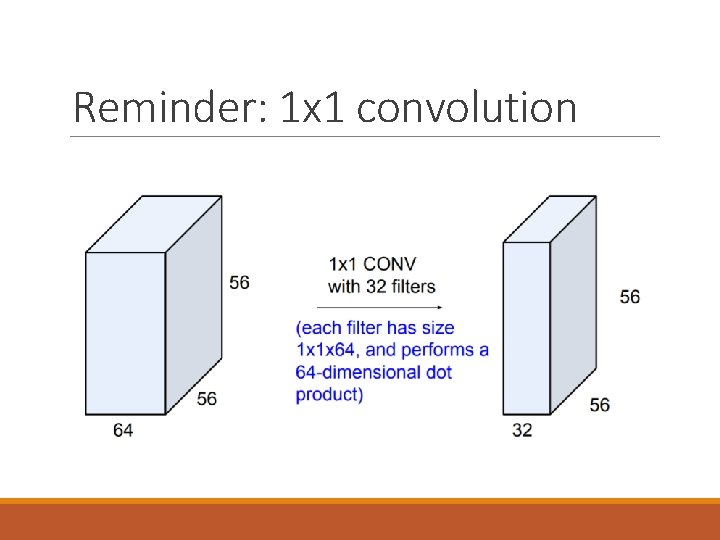
Reminder: 1 x 1 convolution

Google. Net Naïve “Inception” module: Solution: “bottleneck” layers that use 1 x 1 convolutions to reduce feature depth

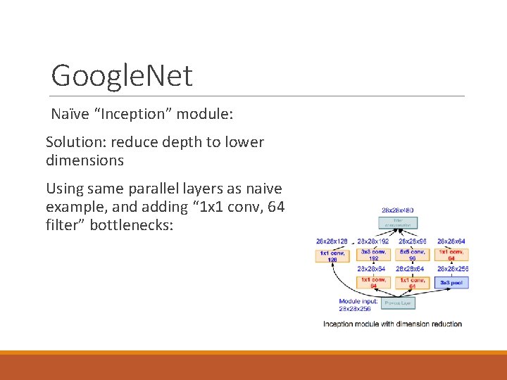
Google. Net Naïve “Inception” module: Solution: reduce depth to lower dimensions Using same parallel layers as naive example, and adding “ 1 x 1 conv, 64 filter” bottlenecks:

Google. Net Naïve “Inception” module: Conv Ops: [1 x 1 conv, 64] 28 x 28 x 64 x 1 x 1 x 256 [1 x 1 conv, 128] 28 x 128 x 1 x 1 x 256 [3 x 3 conv, 192] 28 x 192 x 3 x 3 x 64 [5 x 5 conv, 96] 28 x 96 x 5 x 5 x 64 [1 x 1 conv, 64] 28 x 64 x 1 x 1 x 256 Total: 358 M ops Compared to 854 M ops for naive version Bottleneck can also reduce depth after pooling layer

Google. Net Deeper networks, with computational efficiency

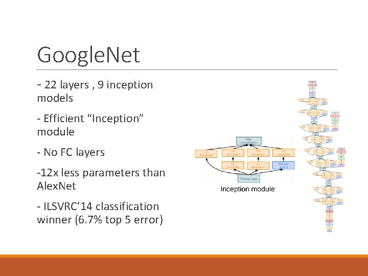
Google. Net - 22 layers , 9 inception models - Efficient “Inception” module - No FC layers -12 x less parameters than Alex. Net - ILSVRC’ 14 classification winner (6. 7% top 5 error)

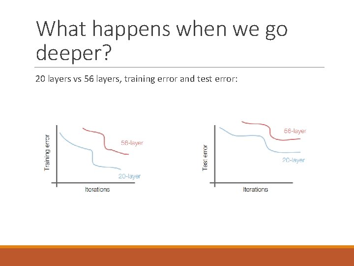
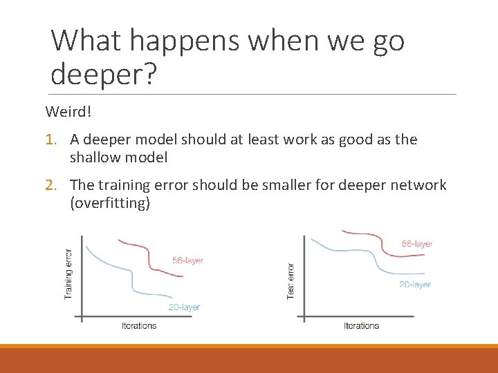
What happens when we go deeper? 20 layers vs 56 layers, training error and test error:

What happens when we go deeper? Weird! 1. A deeper model should at least work as good as the shallow model 2. The training error should be smaller for deeper network (overfitting)

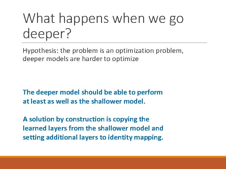
What happens when we go deeper? Hypothesis: the problem is an optimization problem, deeper models are harder to optimize The deeper model should be able to perform at least as well as the shallower model. A solution by construction is copying the learned layers from the shallower model and setting additional layers to identity mapping.

Image. Net Large Scale Visual Recognition Challenge (ILSVRC) winners

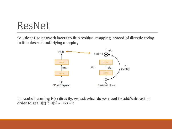
Res. Net Solution: Use network layers to fit a residual mapping instead of directly trying to fit a desired underlying mapping Instead of learning H(x) directly, we ask what do we need to add/subtract in order to get H(x) ? H(x) = F(x) + x

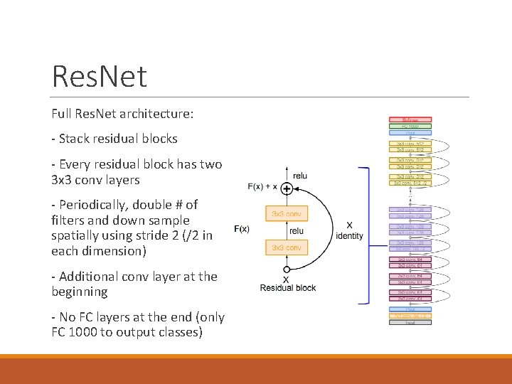
Res. Net Full Res. Net architecture: - Stack residual blocks - Every residual block has two 3 x 3 conv layers - Periodically, double # of filters and down sample spatially using stride 2 (/2 in each dimension) - Additional conv layer at the beginning - No FC layers at the end (only FC 1000 to output classes)

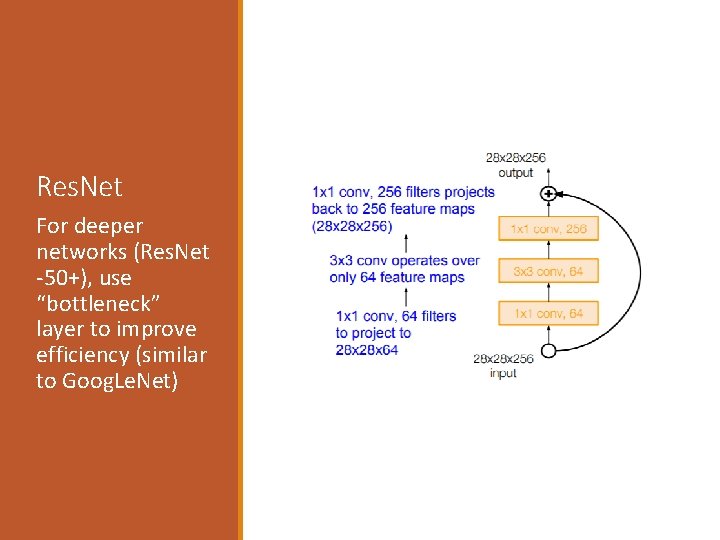
Res. Net For deeper networks (Res. Net -50+), use “bottleneck” layer to improve efficiency (similar to Goog. Le. Net)

Res. Net Training Res. Net in practice: - Batch Normalization after every CONV layer - Xavier/2 initialization from He et al. - SGD + Momentum (0. 9) - Learning rate: 0. 1, divided by 10 when validation error plateaus - Mini-batch size 256 - Weight decay of 1 e-5 - No dropout used

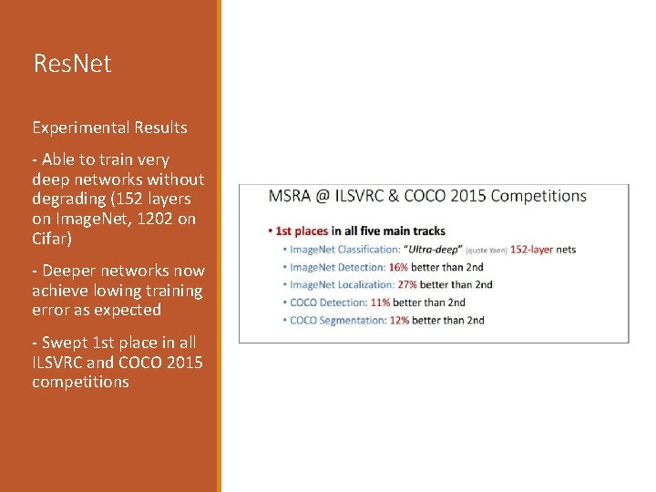
Res. Net Experimental Results - Able to train very deep networks without degrading (152 layers on Image. Net, 1202 on Cifar) - Deeper networks now achieve lowing training error as expected - Swept 1 st place in all ILSVRC and COCO 2015 competitions