Image segmentation 2015160035 1 Image segmentation 4 Result

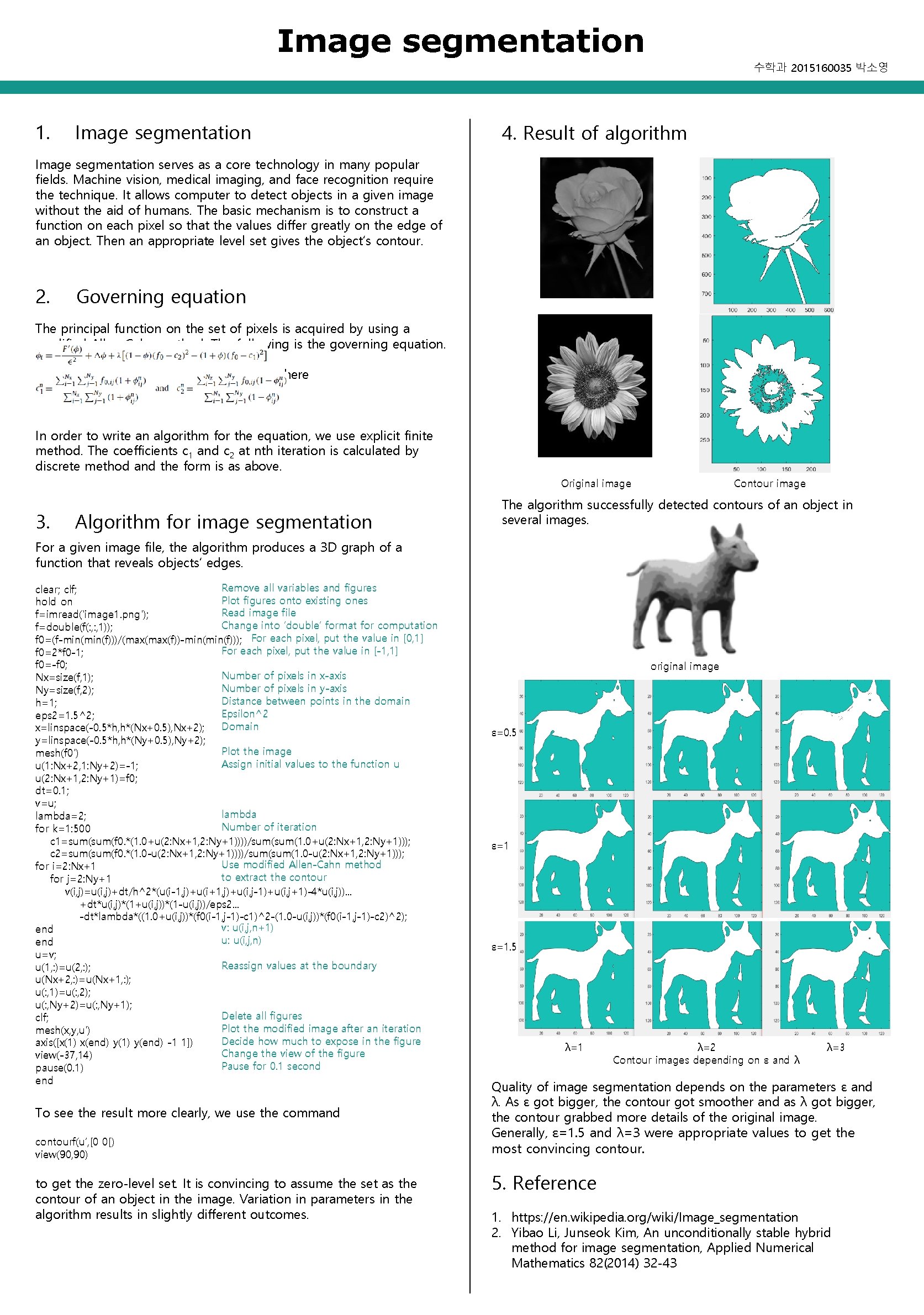
Image segmentation 수학과 2015160035 박소영 1. Image segmentation 4. Result of algorithm Image segmentation serves as a core technology in many popular fields. Machine vision, medical imaging, and face recognition require the technique. It allows computer to detect objects in a given image without the aid of humans. The basic mechanism is to construct a function on each pixel so that the values differ greatly on the edge of an object. Then an appropriate level set gives the object’s contour. 2. Governing equation The principal function on the set of pixels is acquired by using a modified Allen-Cahn method. The following is the governing equation. where In order to write an algorithm for the equation, we use explicit finite method. The coefficients c 1 and c 2 at nth iteration is calculated by discrete method and the form is as above. Original image 3. Algorithm for image segmentation Contour image The algorithm successfully detected contours of an object in several images. For a given image file, the algorithm produces a 3 D graph of a function that reveals objects’ edges. Remove all variables and figures clear; clf; Plot figures onto existing ones hold on Read image file f=imread('image 1. png'); Change into ‘double’ format for computation f=double(f(: , 1)); f 0=(f-min(f)))/(max(f))-min(f))); For each pixel, put the value in [0, 1] For each pixel, put the value in [-1, 1] f 0=2*f 0 -1; f 0=-f 0; Number of pixels in x-axis Nx=size(f, 1); Number of pixels in y-axis Ny=size(f, 2); Distance between points in the domain h=1; Epsilon^2 eps 2=1. 5^2; Domain x=linspace(-0. 5*h, h*(Nx+0. 5), Nx+2); y=linspace(-0. 5*h, h*(Ny+0. 5), Ny+2); Plot the image mesh(f 0') Assign initial values to the function u u(1: Nx+2, 1: Ny+2)=-1; u(2: Nx+1, 2: Ny+1)=f 0; dt=0. 1; v=u; lambda=2; Number of iteration for k=1: 500 c 1=sum(f 0. *(1. 0+u(2: Nx+1, 2: Ny+1))))/sum(1. 0+u(2: Nx+1, 2: Ny+1))); c 2=sum(f 0. *(1. 0 -u(2: Nx+1, 2: Ny+1))))/sum(1. 0 -u(2: Nx+1, 2: Ny+1))); Use modified Allen-Cahn method for i=2: Nx+1 to extract the contour for j=2: Ny+1 v(i, j)=u(i, j)+dt/h^2*(u(i-1, j)+u(i+1, j)+u(i, j-1)+u(i, j+1)-4*u(i, j)). . . +dt*u(i, j)*(1+u(i, j))*(1 -u(i, j))/eps 2. . . -dt*lambda*((1. 0+u(i, j))*(f 0(i-1, j-1)-c 1)^2 -(1. 0 -u(i, j))*(f 0(i-1, j-1)-c 2)^2); v: u(i, j, n+1) end u: u(i, j, n) end u=v; Reassign values at the boundary u(1, : )=u(2, : ); u(Nx+2, : )=u(Nx+1, : ); u(: , 1)=u(: , 2); u(: , Ny+2)=u(: , Ny+1); Delete all figures clf; Plot the modified image after an iteration mesh(x, y, u') Decide how much to expose in the figure axis([x(1) x(end) y(1) y(end) -1 1]) Change the view of the figure view(-37, 14) Pause for 0. 1 second pause(0. 1) end To see the result more clearly, we use the command contourf(u’, [0 0[) view(90, 90) to get the zero-level set. It is convincing to assume the set as the contour of an object in the image. Variation in parameters in the algorithm results in slightly different outcomes. original image ε=0. 5 ε=1. 5 λ=1 λ=2 Contour images depending on ε and λ λ=3 Quality of image segmentation depends on the parameters ε and λ. As ε got bigger, the contour got smoother and as λ got bigger, the contour grabbed more details of the original image. Generally, ε=1. 5 and λ=3 were appropriate values to get the most convincing contour. 5. Reference 1. https: //en. wikipedia. org/wiki/Image_segmentation 2. Yibao Li, Junseok Kim, An unconditionally stable hybrid method for image segmentation, Applied Numerical Mathematics 82(2014) 32 -43