Forecasting Demand 4 Power Point presentation to accompany

Forecasting Demand 4 Power. Point presentation to accompany Heizer and Render Operations Management, Global Edition, Eleventh Edition Principles of Operations Management, Global Edition, Ninth Edition Power. Point slides by Jeff Heyl © 2014 Pearson Education 4 -1

Outline ▶ What is Forecasting? ▶ Forecasting Approaches ü Qualitative Methods ü Quantitative Methods © 2014 Pearson Education ▶ Naive Approach ▶ Moving Averages ▶ Exponential Smoothing with Trend Adjustment ▶ Trend Projections ▶ Seasonal Variations in Data ▶ Linear Regression 4 -2

What is Forecasting? ► ► Process of predicting a future event Underlying basis of all business decisions ► Production ► Inventory ► Personnel ► Facilities © 2014 Pearson Education ? ? 4 -3

Forecasting Time Horizons 1. Short-range forecast ► ► ► 2. 3. Up to 1 year, generally less than 3 months Purchasing, job scheduling, workforce levels, job assignments, production levels Tend to be more accurate than longer-term forecasts Medium-range forecast ► 3 months to 3 years ► Sales and production planning, budgeting Long-range forecast ► 3+ years ► New product planning, facility location, research development © 2014 Pearson Education and 4 -4

The Realities! ► ► ► Forecasts are seldom perfect, unpredictable outside factors may impact the forecast Most techniques assume an underlying stability in the system Product family and aggregated forecasts are more accurate than individual product forecasts © 2014 Pearson Education 4 -5

Forecasting Approaches Qualitative Forecasting ► ► Used when situation is vague and little data such as new products, new technology Involves intuition, experience Quantitative Forecasting ► ► Used when situation is ‘stable’ and historical data exist ► Existing products ► Current technology Involves mathematical techniques ► e. g. , forecasting sales of color televisions © 2014 Pearson Education 4 -6

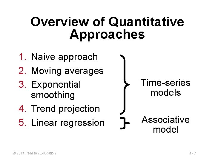
Overview of Quantitative Approaches 1. Naive approach 2. Moving averages 3. Exponential smoothing 4. Trend projection 5. Linear regression © 2014 Pearson Education Time-series models Associative model 4 -7

Time-Series Forecasting ► Set of evenly spaced numerical data ► ► Obtained by observing response variable at regular time periods Forecast based only on past values, no other variables important ► Assumes that factors influencing past and present will continue influence in future © 2014 Pearson Education 4 -8

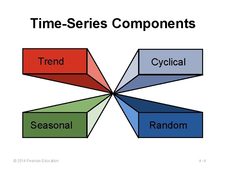
Time-Series Components Trend Cyclical Seasonal Random © 2014 Pearson Education 4 -9

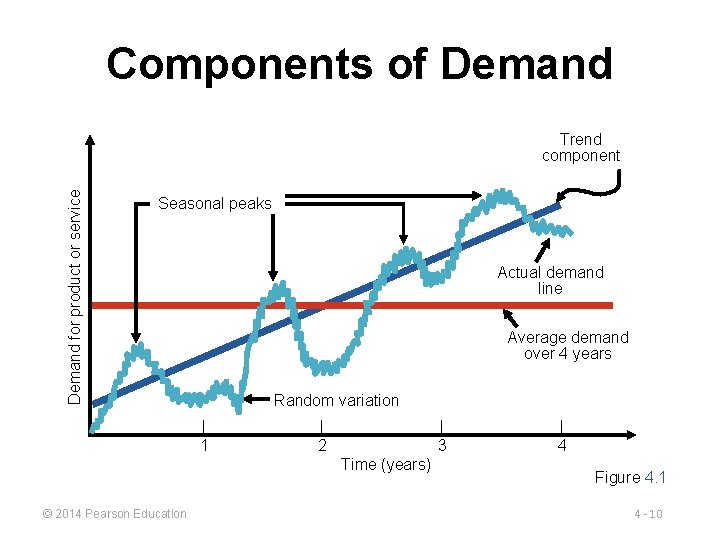
Components of Demand for product or service Trend component Seasonal peaks Actual demand line Average demand over 4 years Random variation | 1 | 2 | 3 Time (years) © 2014 Pearson Education | 4 Figure 4. 1 4 - 10

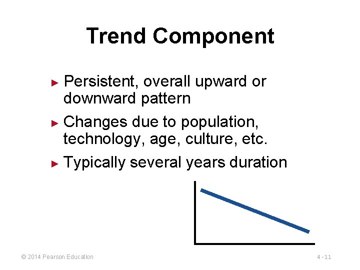
Trend Component Persistent, overall upward or downward pattern ► Changes due to population, technology, age, culture, etc. ► Typically several years duration ► © 2014 Pearson Education 4 - 11

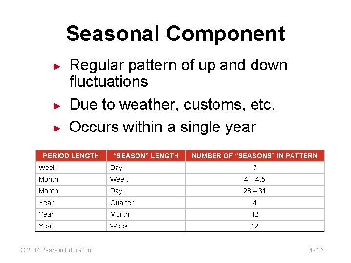
Seasonal Component ► ► ► Regular pattern of up and down fluctuations Due to weather, customs, etc. Occurs within a single year PERIOD LENGTH “SEASON” LENGTH NUMBER OF “SEASONS” IN PATTERN Week Day Month Week 4 – 4. 5 Month Day 28 – 31 Year Quarter 4 Year Month 12 Year Week 52 © 2014 Pearson Education 7 4 - 12

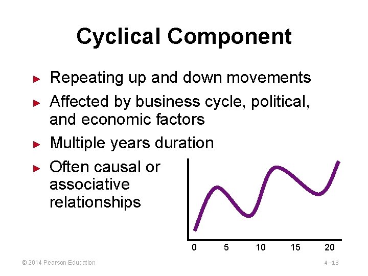
Cyclical Component ► ► Repeating up and down movements Affected by business cycle, political, and economic factors Multiple years duration Often causal or associative relationships 0 © 2014 Pearson Education 5 10 15 20 4 - 13

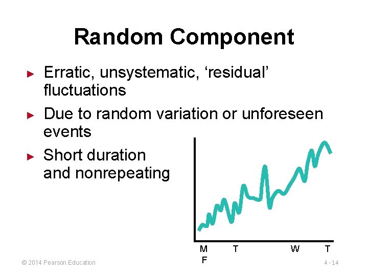
Random Component ► ► ► Erratic, unsystematic, ‘residual’ fluctuations Due to random variation or unforeseen events Short duration and nonrepeating © 2014 Pearson Education M F T W T 4 - 14

Naive Approach ► Assumes demand in next period is the same as demand in most recent period ► ► ► e. g. , If January sales were 68, then February sales will be 68 Sometimes cost effective and efficient Can be good starting point © 2014 Pearson Education 4 - 15

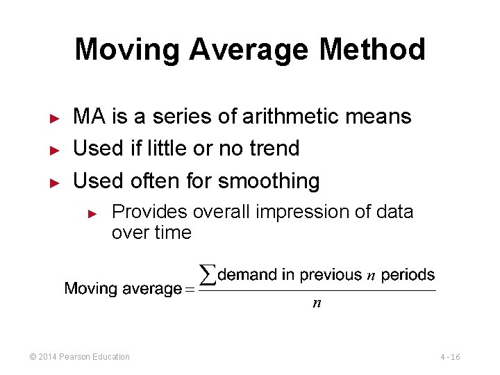
Moving Average Method ► ► ► MA is a series of arithmetic means Used if little or no trend Used often for smoothing ► Provides overall impression of data over time © 2014 Pearson Education 4 - 16

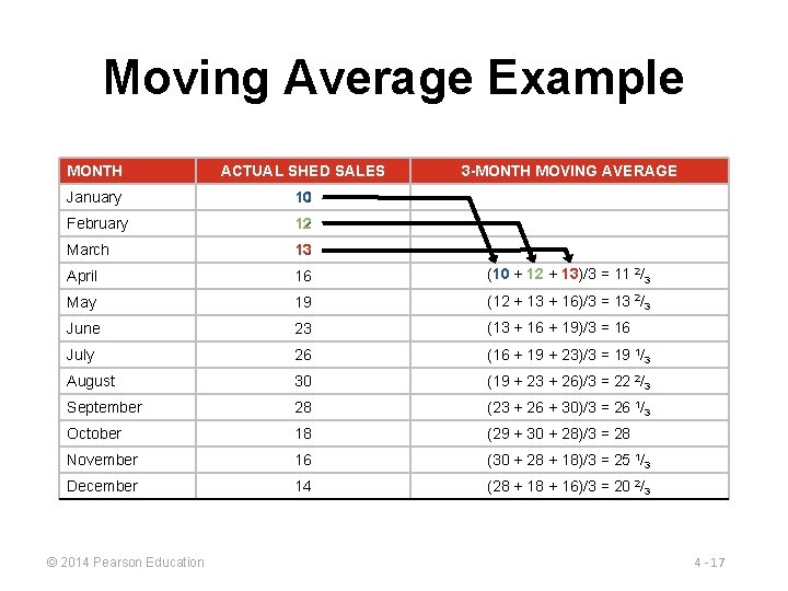
Moving Average Example MONTH ACTUAL SHED SALES January 10 February 12 March 13 April 16 (10 + 12 + 13)/3 = 11 2/3 May 19 (12 + 13 + 16)/3 = 13 2/3 June 23 (13 + 16 + 19)/3 = 16 July 26 (16 + 19 + 23)/3 = 19 1/3 August 30 (19 + 23 + 26)/3 = 22 2/3 September 28 (23 + 26 + 30)/3 = 26 1/3 October 18 (29 + 30 + 28)/3 = 28 November 16 (30 + 28 + 18)/3 = 25 1/3 December 14 (28 + 16)/3 = 20 2/3 © 2014 Pearson Education 3 -MONTH MOVING AVERAGE 4 - 17

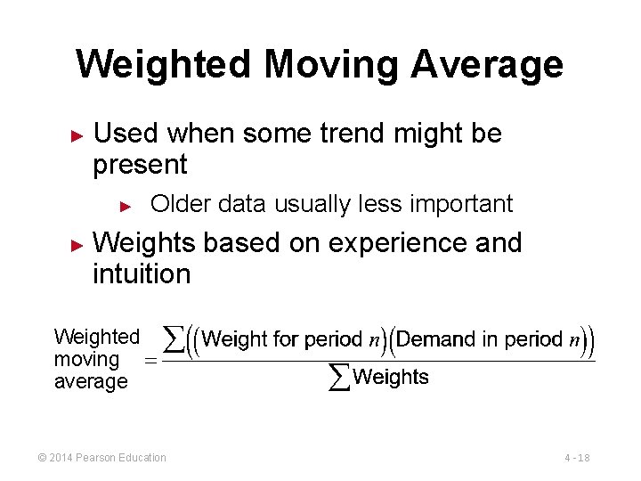
Weighted Moving Average ► Used when some trend might be present ► ► Older data usually less important Weights based on experience and intuition Weighted moving average © 2014 Pearson Education 4 - 18

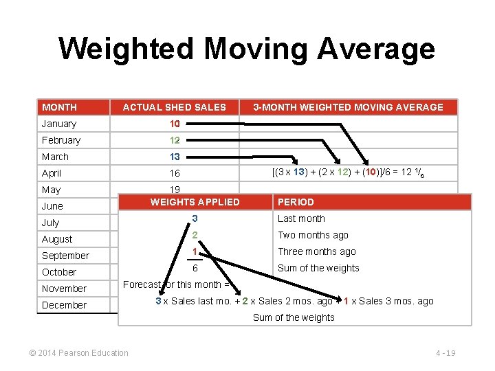
Weighted Moving Average MONTH ACTUAL SHED SALES January 10 February 12 March 13 April 16 May [(3 x 13) + (2 x 12) + (10)]/6 = 12 1/6 19 WEIGHTS APPLIED 23 June 3 -MONTH WEIGHTED MOVING AVERAGE PERIOD July 26 3 Last month August 30 2 Two months ago September 28 1 Three months ago October November 18 6 Forecast for 16 this month = December Sum of the weights 3 x 14 Sales last mo. + 2 x Sales 2 mos. ago + 1 x Sales 3 mos. ago Sum of the weights © 2014 Pearson Education 4 - 19

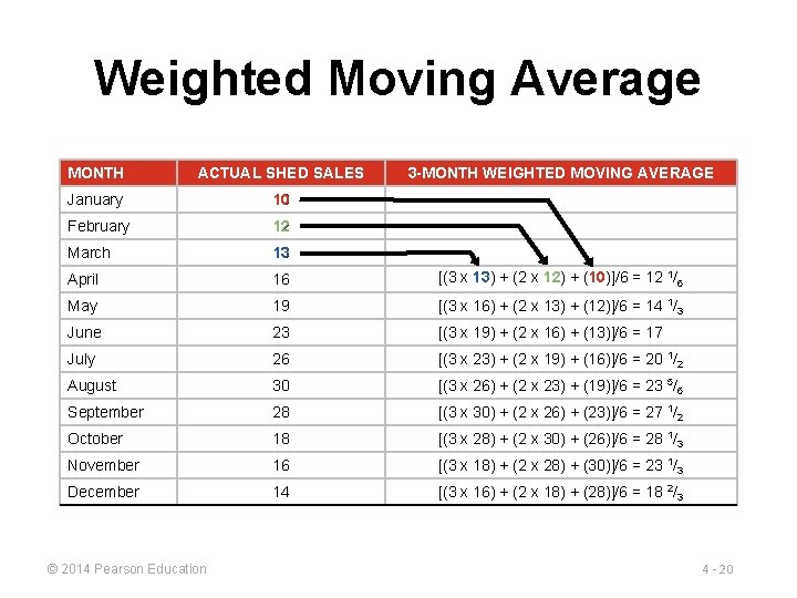
Weighted Moving Average MONTH ACTUAL SHED SALES January 10 February 12 March 13 April 16 [(3 x 13) + (2 x 12) + (10)]/6 = 12 1/6 May 19 [(3 x 16) + (2 x 13) + (12)]/6 = 14 1/3 June 23 [(3 x 19) + (2 x 16) + (13)]/6 = 17 July 26 [(3 x 23) + (2 x 19) + (16)]/6 = 20 1/2 August 30 [(3 x 26) + (2 x 23) + (19)]/6 = 23 5/6 September 28 [(3 x 30) + (2 x 26) + (23)]/6 = 27 1/2 October 18 [(3 x 28) + (2 x 30) + (26)]/6 = 28 1/3 November 16 [(3 x 18) + (2 x 28) + (30)]/6 = 23 1/3 December 14 [(3 x 16) + (2 x 18) + (28)]/6 = 18 2/3 © 2014 Pearson Education 3 -MONTH WEIGHTED MOVING AVERAGE 4 - 20

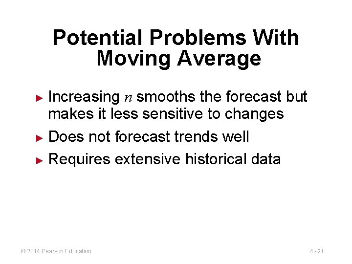
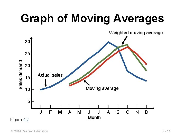
Potential Problems With Moving Average Increasing n smooths the forecast but makes it less sensitive to changes ► Does not forecast trends well ► Requires extensive historical data ► © 2014 Pearson Education 4 - 21

Graph of Moving Averages Weighted moving average 30 – Sales demand 25 – 20 – 15 – Actual sales Moving average 10 – 5– | | | J F M A M Figure 4. 2 © 2014 Pearson Education | | J J Month | | | A S O N D 4 - 22

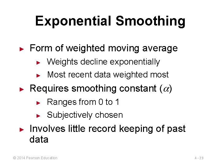
Exponential Smoothing ► ► ► Form of weighted moving average ► Weights decline exponentially ► Most recent data weighted most Requires smoothing constant ( ) ► Ranges from 0 to 1 ► Subjectively chosen Involves little record keeping of past data © 2014 Pearson Education 4 - 23

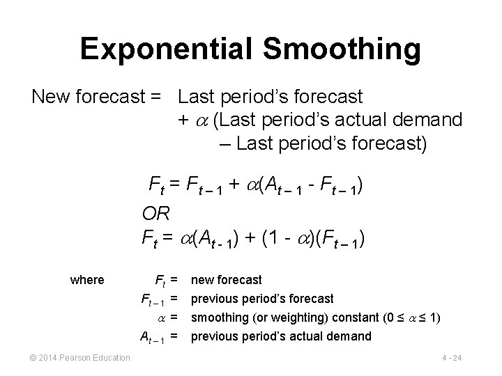
Exponential Smoothing New forecast = Last period’s forecast + (Last period’s actual demand – Last period’s forecast) Ft = Ft – 1 + (At – 1 - Ft – 1) OR Ft = (At - 1) + (1 - )(Ft – 1) where © 2014 Pearson Education Ft = new forecast Ft – 1 = = previous period’s forecast smoothing (or weighting) constant (0 ≤ ≤ 1) At – 1 = previous period’s actual demand 4 - 24

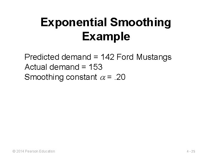
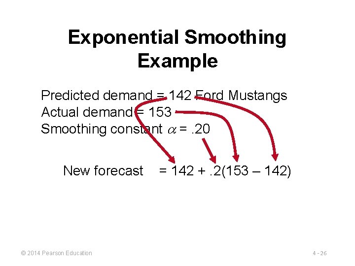
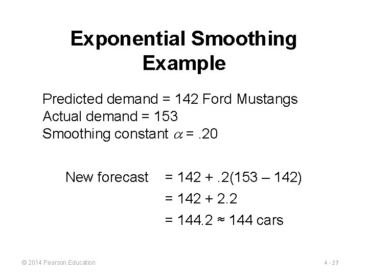
Exponential Smoothing Example Predicted demand = 142 Ford Mustangs Actual demand = 153 Smoothing constant =. 20 © 2014 Pearson Education 4 - 25

Exponential Smoothing Example Predicted demand = 142 Ford Mustangs Actual demand = 153 Smoothing constant =. 20 New forecast © 2014 Pearson Education = 142 +. 2(153 – 142) 4 - 26

Exponential Smoothing Example Predicted demand = 142 Ford Mustangs Actual demand = 153 Smoothing constant =. 20 New forecast = 142 +. 2(153 – 142) = 142 + 2. 2 = 144. 2 ≈ 144 cars © 2014 Pearson Education 4 - 27

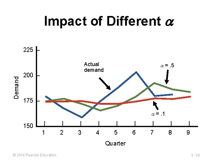
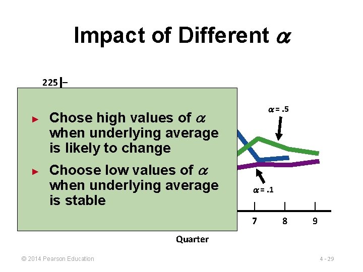
Impact of Different Demand 225 – Actual demand 200 – =. 5 175 – =. 1 150 – | 1 | 2 | 3 | 4 | 5 | 6 | 7 | 8 | 9 Quarter © 2014 Pearson Education 4 - 28

Impact of Different 225 – Demand ► Actual demand values =. 5 Chose high of when underlying average is likely to change 200 – Choose low values of when underlying average is stable | | | ► 175 – 150 – 1 2 3 4 5 6 =. 1 | | | 7 8 9 Quarter © 2014 Pearson Education 4 - 29

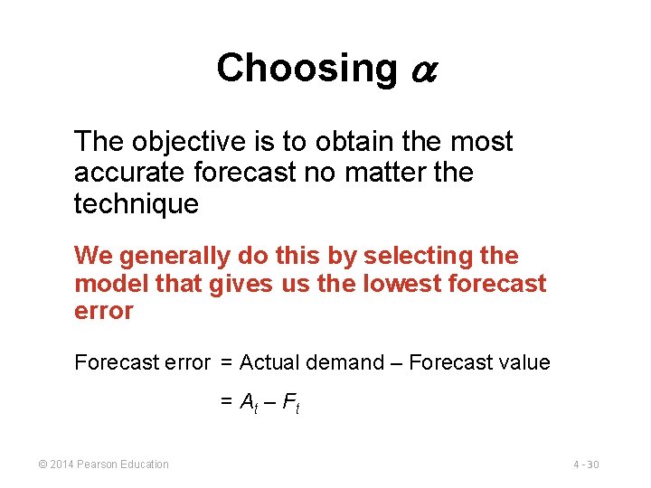
Choosing The objective is to obtain the most accurate forecast no matter the technique We generally do this by selecting the model that gives us the lowest forecast error Forecast error = Actual demand – Forecast value = At – Ft © 2014 Pearson Education 4 - 30

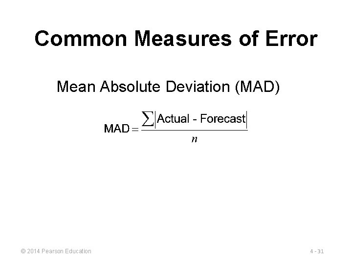
Common Measures of Error Mean Absolute Deviation (MAD) © 2014 Pearson Education 4 - 31

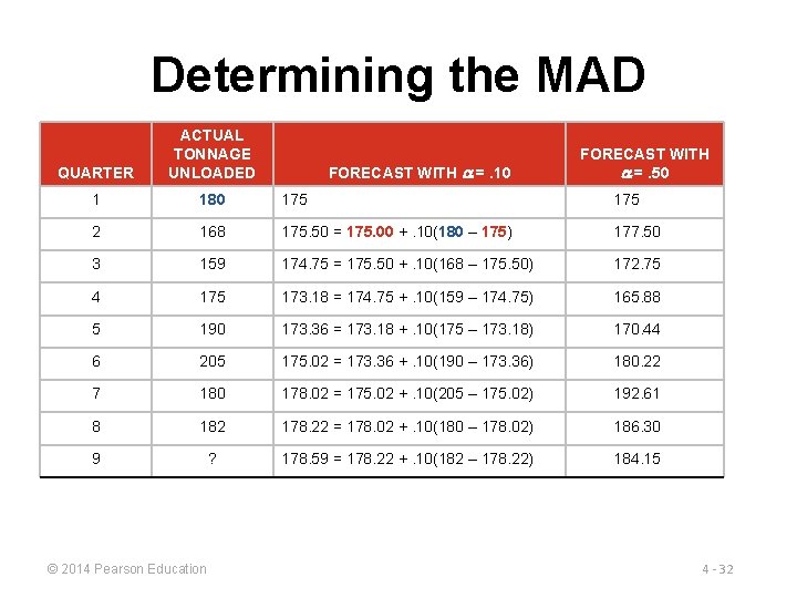
Determining the MAD QUARTER ACTUAL TONNAGE UNLOADED 1 180 175 2 168 175. 50 = 175. 00 +. 10(180 – 175) 177. 50 3 159 174. 75 = 175. 50 +. 10(168 – 175. 50) 172. 75 4 175 173. 18 = 174. 75 +. 10(159 – 174. 75) 165. 88 5 190 173. 36 = 173. 18 +. 10(175 – 173. 18) 170. 44 6 205 175. 02 = 173. 36 +. 10(190 – 173. 36) 180. 22 7 180 178. 02 = 175. 02 +. 10(205 – 175. 02) 192. 61 8 182 178. 22 = 178. 02 +. 10(180 – 178. 02) 186. 30 9 ? 178. 59 = 178. 22 +. 10(182 – 178. 22) 184. 15 © 2014 Pearson Education FORECAST WITH =. 10 FORECAST WITH =. 50 4 - 32

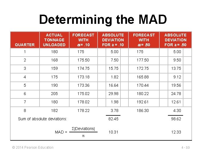
Determining the MAD QUARTER ACTUAL TONNAGE UNLOADED FORECAST WITH =. 10 1 180 175 5. 00 2 168 175. 50 7. 50 177. 50 9. 50 3 159 174. 75 15. 75 172. 75 13. 75 4 175 173. 18 1. 82 165. 88 9. 12 5 190 173. 36 16. 64 170. 44 19. 56 6 205 175. 02 29. 98 180. 22 24. 78 7 180 178. 02 1. 98 192. 61 12. 61 8 182 178. 22 3. 78 186. 30 4. 30 Sum of absolute deviations: MAD = © 2014 Pearson Education Σ|Deviations| n ABSOLUTE DEVIATION FOR a =. 10 FORECAST WITH =. 50 ABSOLUTE DEVIATION FOR a =. 50 82. 45 98. 62 10. 31 12. 33 4 - 33

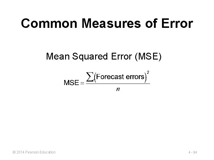
Common Measures of Error Mean Squared Error (MSE) © 2014 Pearson Education 4 - 34

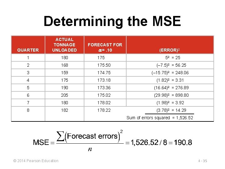
Determining the MSE QUARTER ACTUAL TONNAGE UNLOADED 1 180 175 2 168 175. 50 (– 7. 5)2 = 56. 25 3 159 174. 75 (– 15. 75)2 = 248. 06 4 175 173. 18 (1. 82)2 = 3. 31 5 190 173. 36 (16. 64)2 = 276. 89 6 205 175. 02 (29. 98)2 = 898. 80 7 180 178. 02 (1. 98)2 = 3. 92 8 182 178. 22 (3. 78)2 = 14. 29 FORECAST FOR =. 10 (ERROR)2 52 = 25 Sum of errors squared = 1, 526. 52 © 2014 Pearson Education 4 - 35

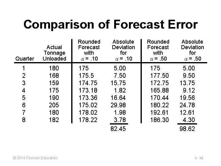
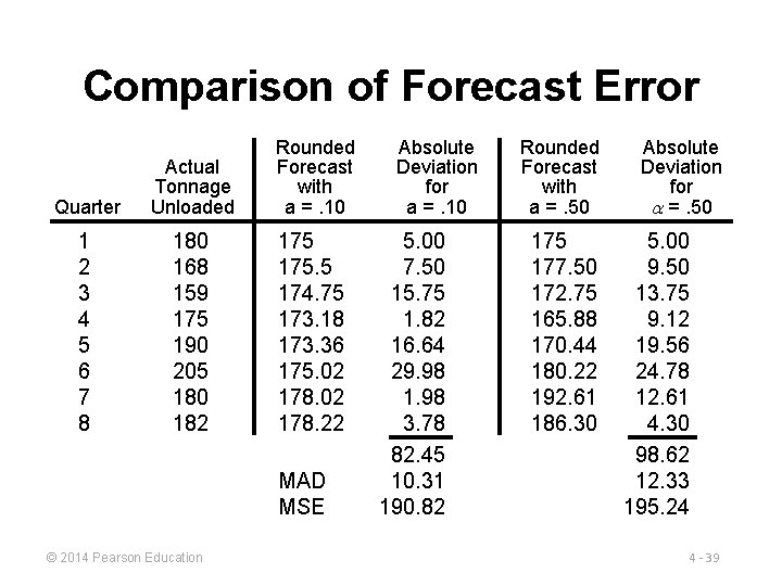
Comparison of Forecast Error Quarter Actual Tonnage Unloaded Rounded Forecast with =. 10 Absolute Deviation for =. 10 1 2 3 4 5 6 7 8 180 168 159 175 190 205 180 182 175. 5 174. 75 173. 18 173. 36 175. 02 178. 22 5. 00 7. 50 15. 75 1. 82 16. 64 29. 98 1. 98 3. 78 82. 45 © 2014 Pearson Education Rounded Forecast with =. 50 175 177. 50 172. 75 165. 88 170. 44 180. 22 192. 61 186. 30 Absolute Deviation for =. 50 5. 00 9. 50 13. 75 9. 12 19. 56 24. 78 12. 61 4. 30 98. 62 4 - 36

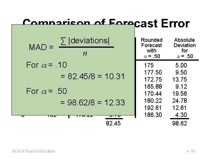
Comparison of Forecast Error Rounded Absolute ∑ |deviations| Actual Forecast Deviation MAD = Tonnage with for n Quarter Unloaded a =. 10 1 For 180 5. 00 =. 10 175 2 168 175. 5 7. 50 3 159 = 82. 45/8 174. 75 = 10. 31 15. 75 4 5 For 6 7 8 175 173. 18 190 =. 50 173. 36 205 = 98. 62/8 175. 02 180 178. 02 182 178. 22 © 2014 Pearson Education = 1. 82 16. 64 29. 98 12. 33 1. 98 3. 78 82. 45 Rounded Forecast with =. 50 175 177. 50 172. 75 165. 88 170. 44 180. 22 192. 61 186. 30 Absolute Deviation for =. 50 5. 00 9. 50 13. 75 9. 12 19. 56 24. 78 12. 61 4. 30 98. 62 4 - 37

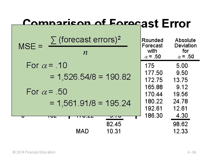
Comparison of Forecast Error 2 Rounded Absolute ∑ (forecast errors) Actual Forecast Deviation MSE =Tonnage with for n Quarter Unloaded a =. 10 1 For 2 3 4 5 For 6 7 8 180 =. 10 175 168 175. 5 = 1, 526. 54/8 159 174. 75 173. 18 190 =. 50 173. 36 205 175. 02 = 1, 561. 91/8 180 178. 02 182 178. 22 MAD © 2014 Pearson Education = = 5. 00 7. 50 190. 82 15. 75 1. 82 16. 64 29. 98 195. 24 1. 98 3. 78 82. 45 10. 31 Rounded Forecast with =. 50 175 177. 50 172. 75 165. 88 170. 44 180. 22 192. 61 186. 30 Absolute Deviation for =. 50 5. 00 9. 50 13. 75 9. 12 19. 56 24. 78 12. 61 4. 30 98. 62 12. 33 4 - 38

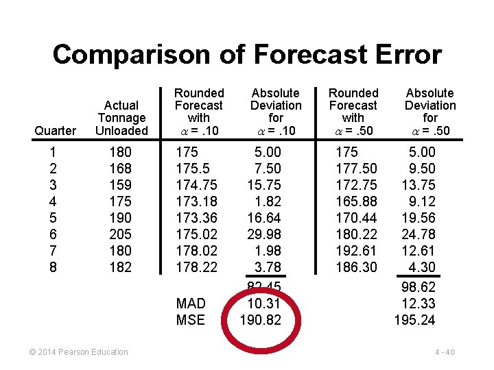
Comparison of Forecast Error Quarter Actual Tonnage Unloaded Rounded Forecast with a =. 10 1 2 3 4 5 6 7 8 180 168 159 175 190 205 180 182 175. 5 174. 75 173. 18 173. 36 175. 02 178. 22 MAD MSE © 2014 Pearson Education Absolute Deviation for a =. 10 5. 00 7. 50 15. 75 1. 82 16. 64 29. 98 1. 98 3. 78 82. 45 10. 31 190. 82 Rounded Forecast with a =. 50 175 177. 50 172. 75 165. 88 170. 44 180. 22 192. 61 186. 30 Absolute Deviation for =. 50 5. 00 9. 50 13. 75 9. 12 19. 56 24. 78 12. 61 4. 30 98. 62 12. 33 195. 24 4 - 39

Comparison of Forecast Error Quarter Actual Tonnage Unloaded Rounded Forecast with =. 10 1 2 3 4 5 6 7 8 180 168 159 175 190 205 180 182 175. 5 174. 75 173. 18 173. 36 175. 02 178. 22 MAD MSE © 2014 Pearson Education Absolute Deviation for =. 10 5. 00 7. 50 15. 75 1. 82 16. 64 29. 98 1. 98 3. 78 82. 45 10. 31 190. 82 Rounded Forecast with =. 50 175 177. 50 172. 75 165. 88 170. 44 180. 22 192. 61 186. 30 Absolute Deviation for =. 50 5. 00 9. 50 13. 75 9. 12 19. 56 24. 78 12. 61 4. 30 98. 62 12. 33 195. 24 4 - 40

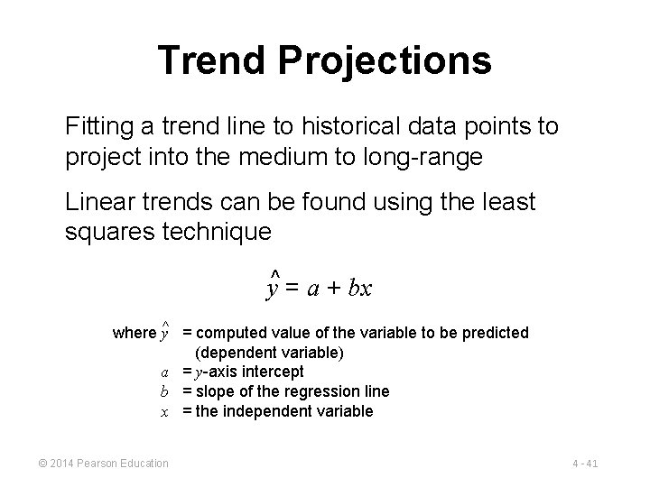
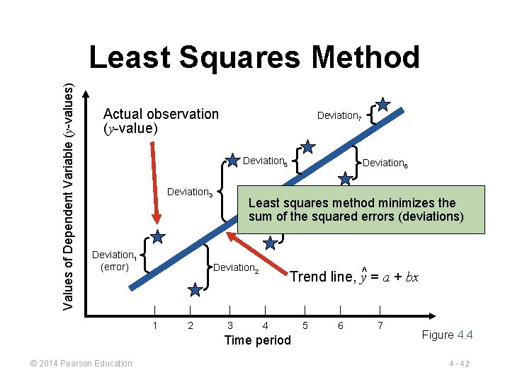
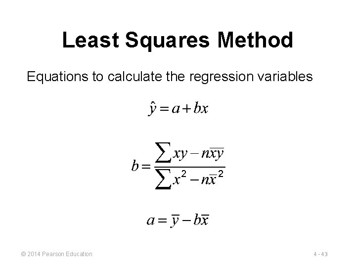
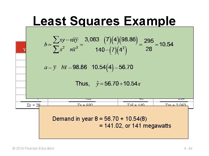
Trend Projections Fitting a trend line to historical data points to project into the medium to long-range Linear trends can be found using the least squares technique y^ = a + bx where y^ = computed value of the variable to be predicted (dependent variable) a = y-axis intercept b = slope of the regression line x = the independent variable © 2014 Pearson Education 4 - 41

Values of Dependent Variable (y-values) Least Squares Method Actual observation (y-value) Deviation 7 Deviation 5 Deviation 3 Deviation 1 (error) Deviation 6 Least squares method minimizes the sum of Deviation the squared errors (deviations) 4 Deviation 2 Trend line, y^ = a + bx | | | | 1 2 3 4 5 6 7 Time period © 2014 Pearson Education Figure 4. 4 4 - 42

Least Squares Method Equations to calculate the regression variables © 2014 Pearson Education 4 - 43

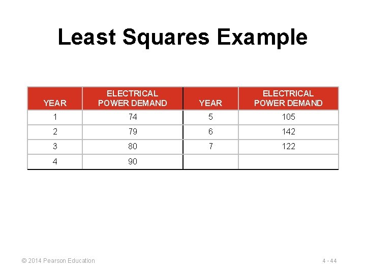
Least Squares Example YEAR ELECTRICAL POWER DEMAND 1 74 5 105 2 79 6 142 3 80 7 122 4 90 © 2014 Pearson Education 4 - 44

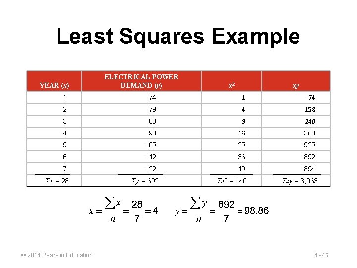
Least Squares Example YEAR (x) ELECTRICAL POWER DEMAND (y) x 2 xy 1 74 2 79 4 158 3 80 9 240 4 90 16 360 5 105 25 525 6 142 36 852 7 122 49 854 Σx = 28 © 2014 Pearson Education Σy = 692 Σx 2 = 140 Σxy = 3, 063 4 - 45

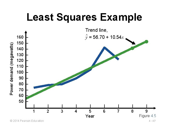
Least Squares Example ELECTRICAL POWER DEMAND (y) YEAR (x) x 2 xy 1 74 2 79 4 158 3 80 9 240 4 90 16 360 5 105 25 525 6 142 36 852 7 122 49 854 Σx = 28 Σy = 692 Σx 2 = 140 Σxy = 3, 063 Demand in year 8 = 56. 70 + 10. 54(8) = 141. 02, or 141 megawatts © 2014 Pearson Education 4 - 46

Power demand (megawatts) Least Squares Example 160 150 140 130 120 110 100 90 80 70 60 50 – – – Trend line, y^ = 56. 70 + 10. 54 x | 1 © 2014 Pearson Education | 2 | 3 | 4 | 5 Year | 6 | 7 | 8 | 9 Figure 4. 5 4 - 47

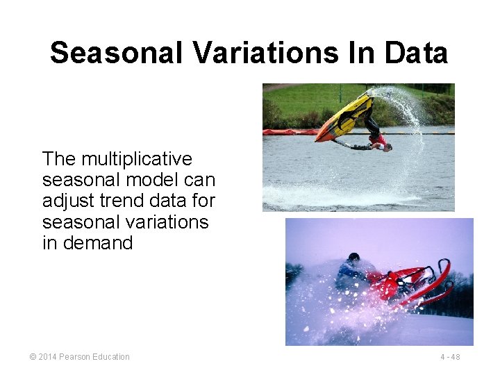
Seasonal Variations In Data The multiplicative seasonal model can adjust trend data for seasonal variations in demand © 2014 Pearson Education 4 - 48

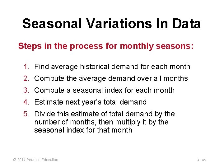
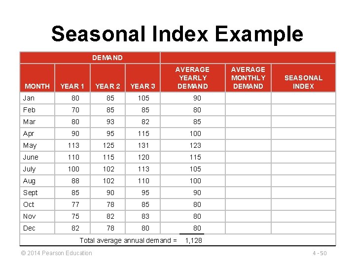
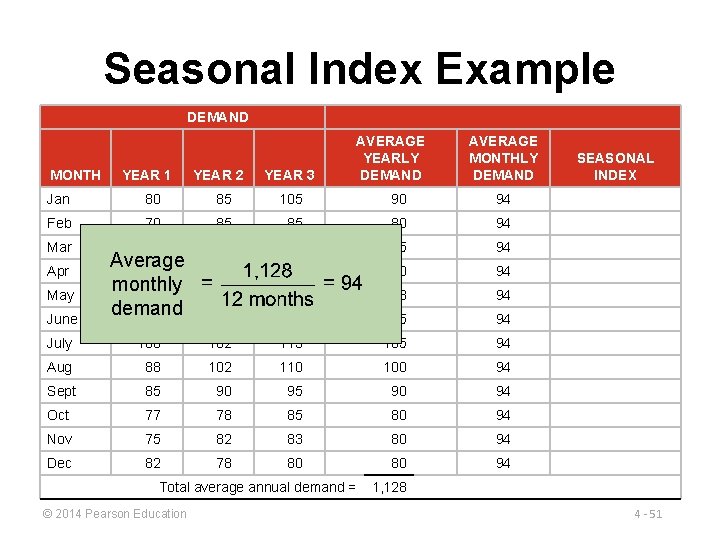
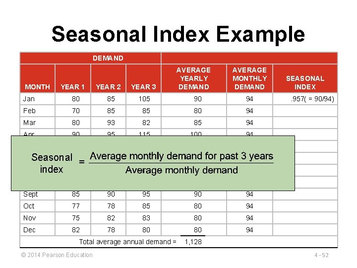
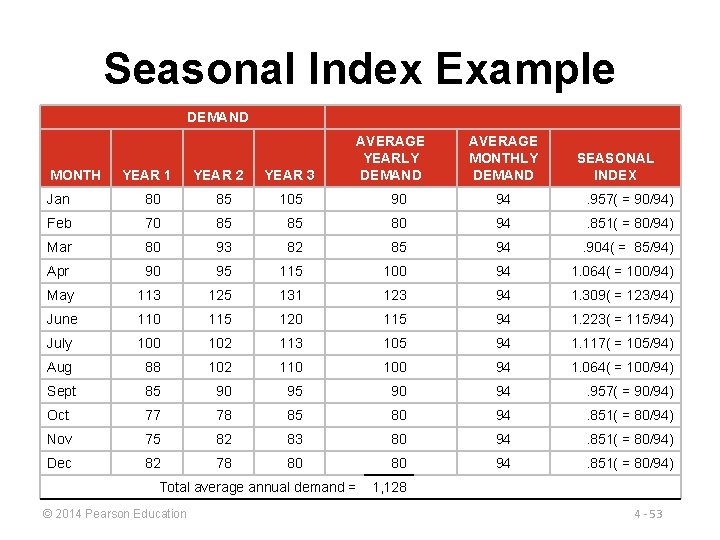
Seasonal Variations In Data Steps in the process for monthly seasons: 1. Find average historical demand for each month 2. Compute the average demand over all months 3. Compute a seasonal index for each month 4. Estimate next year’s total demand 5. Divide this estimate of total demand by the number of months, then multiply it by the seasonal index for that month © 2014 Pearson Education 4 - 49

Seasonal Index Example DEMAND MONTH YEAR 1 YEAR 2 YEAR 3 AVERAGE YEARLY DEMAND Jan 80 85 105 90 Feb 70 85 85 80 Mar 80 93 82 85 Apr 90 95 115 100 May 113 125 131 123 June 110 115 120 115 July 100 102 113 105 Aug 88 102 110 100 Sept 85 90 95 90 Oct 77 78 85 80 Nov 75 82 83 80 Dec 82 78 80 80 Total average annual demand = © 2014 Pearson Education AVERAGE MONTHLY DEMAND SEASONAL INDEX 1, 128 4 - 50

Seasonal Index Example DEMAND MONTH YEAR 1 YEAR 2 YEAR 3 AVERAGE YEARLY DEMAND AVERAGE MONTHLY DEMAND Jan 80 85 105 90 94 Feb 70 85 85 80 94 80 93 82 85 94 95 115 100 94 125 131 123 94 115 120 115 94 Mar June Average 90 monthly 113 demand 110 July 100 102 113 105 94 Aug 88 102 110 100 94 Sept 85 90 94 Oct 77 78 85 80 94 Nov 75 82 83 80 94 Dec 82 78 80 80 94 Apr May Total average annual demand = © 2014 Pearson Education SEASONAL INDEX 1, 128 4 - 51

Seasonal Index Example DEMAND MONTH YEAR 1 YEAR 2 YEAR 3 AVERAGE YEARLY DEMAND AVERAGE MONTHLY DEMAND Jan 80 85 105 90 94 Feb 70 85 85 80 94 Mar 80 93 82 85 94 Apr 90 95 115 100 94 May 113 125 131 123 94 Seasonal 110 June 115 120 115 94 index 100 102 113 105 94 Aug 88 102 110 100 94 Sept 85 90 94 Oct 77 78 85 80 94 Nov 75 82 83 80 94 Dec 82 78 80 80 94 July Total average annual demand = © 2014 Pearson Education SEASONAL INDEX. 957( = 90/94) 1, 128 4 - 52

Seasonal Index Example DEMAND MONTH YEAR 1 YEAR 2 YEAR 3 AVERAGE YEARLY DEMAND AVERAGE MONTHLY DEMAND SEASONAL INDEX Jan 80 85 105 90 94 . 957( = 90/94) Feb 70 85 85 80 94 . 851( = 80/94) Mar 80 93 82 85 94 . 904( = 85/94) Apr 90 95 115 100 94 1. 064( = 100/94) May 113 125 131 123 94 1. 309( = 123/94) June 110 115 120 115 94 1. 223( = 115/94) July 100 102 113 105 94 1. 117( = 105/94) Aug 88 102 110 100 94 1. 064( = 100/94) Sept 85 90 94 . 957( = 90/94) Oct 77 78 85 80 94 . 851( = 80/94) Nov 75 82 83 80 94 . 851( = 80/94) Dec 82 78 80 80 94 . 851( = 80/94) Total average annual demand = © 2014 Pearson Education 1, 128 4 - 53

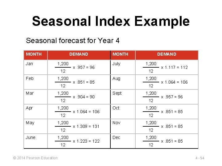
Seasonal Index Example Seasonal forecast for Year 4 MONTH Jan DEMAND 1, 200 12 Feb 1, 200 12 Mar 1, 200 12 Apr 1, 200 12 May 1, 200 12 June 1, 200 12 © 2014 Pearson Education x. 957 = 96 x. 851 = 85 x. 904 = 90 x 1. 064 = 106 x 1. 309 = 131 x 1. 223 = 122 MONTH July DEMAND 1, 200 12 Aug 1, 200 12 Sept 1, 200 12 Oct 1, 200 12 Nov 1, 200 12 Dec 1, 200 12 x 1. 117 = 112 x 1. 064 = 106 x. 957 = 96 x. 851 = 85 4 - 54

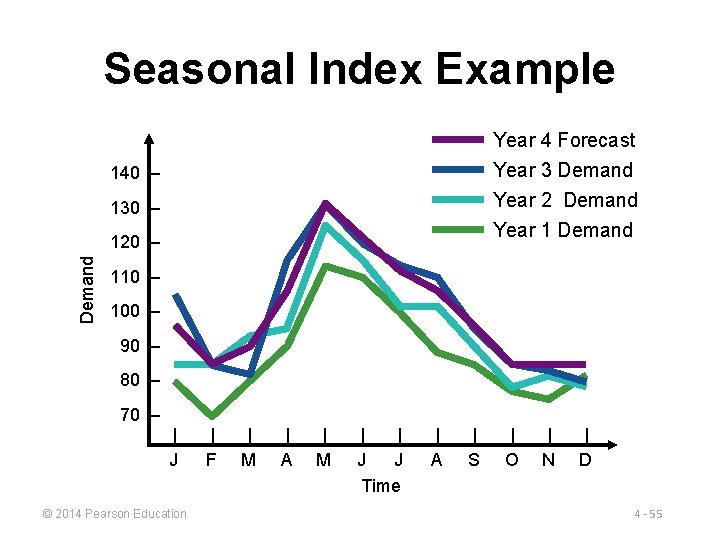
Seasonal Index Example Year 4 Forecast Year 3 Demand Year 2 Demand Year 1 Demand 140 – 130 – Demand 120 – 110 – 100 – 90 – 80 – 70 – | J © 2014 Pearson Education | F | M | A | M | | J J Time | A | S | O | N | D 4 - 55

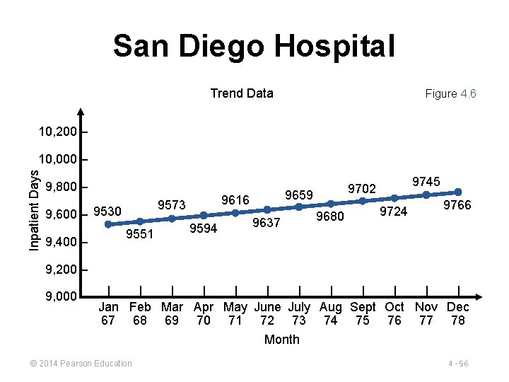
San Diego Hospital Trend Data Figure 4. 6 10, 200 – Inpatient Days 10, 000 – 9, 800 – 9573 9, 600 – 9530 9, 400 – 9551 9659 9616 9594 9637 9745 9702 9680 9724 9766 9, 200 – 9, 000 – | | | Jan Feb Mar Apr May June July Aug Sept Oct Nov Dec 67 68 69 70 71 72 73 74 75 76 77 78 Month © 2014 Pearson Education 4 - 56

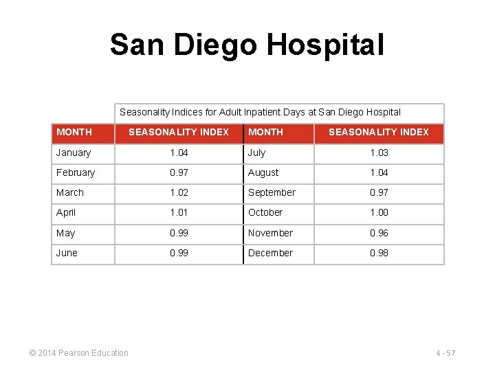
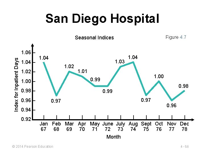
San Diego Hospital Seasonality Indices for Adult Inpatient Days at San Diego Hospital MONTH SEASONALITY INDEX January 1. 04 July 1. 03 February 0. 97 August 1. 04 March 1. 02 September 0. 97 April 1. 01 October 1. 00 May 0. 99 November 0. 96 June 0. 99 December 0. 98 © 2014 Pearson Education MONTH SEASONALITY INDEX 4 - 57

San Diego Hospital Figure 4. 7 Seasonal Indices Index for Inpatient Days 1. 06 – 1. 04 1. 02 – 1. 01 1. 00 0. 99 1. 00 – 0. 98 – 0. 96 – 1. 03 0. 98 0. 99 0. 97 0. 94 – 0. 92 – 1. 04 0. 96 | | | Jan Feb Mar Apr May June July Aug Sept Oct Nov Dec 67 68 69 70 71 72 73 74 75 76 77 78 Month © 2014 Pearson Education 4 - 58

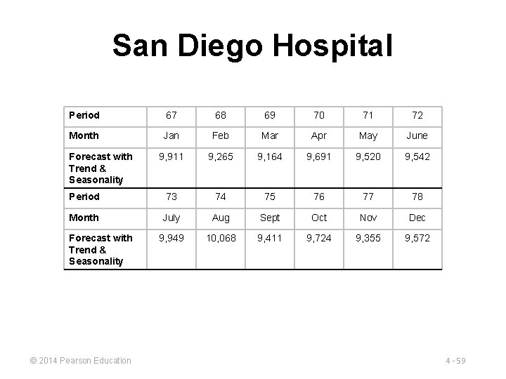
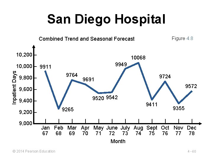
San Diego Hospital Period 67 68 69 70 71 72 Month Jan Feb Mar Apr May June 9, 911 9, 265 9, 164 9, 691 9, 520 9, 542 Period 73 74 75 76 77 78 Month July Aug Sept Oct Nov Dec 9, 949 10, 068 9, 411 9, 724 9, 355 9, 572 Forecast with Trend & Seasonality © 2014 Pearson Education 4 - 59

San Diego Hospital Figure 4. 8 Combined Trend and Seasonal Forecast 10, 200 – 10068 9949 Inpatient Days 10, 000 – 9911 9764 9, 800 – 9724 9691 9572 9, 600 – 9520 9542 9, 400 – 9265 9, 200 – 9, 000 – 9411 9355 | | | Jan Feb Mar Apr May June July Aug Sept Oct Nov Dec 67 68 69 70 71 72 73 74 75 76 77 78 Month © 2014 Pearson Education 4 - 60

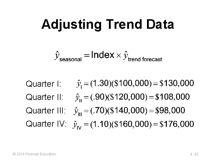
Adjusting Trend Data Quarter I: Quarter III: Quarter IV: © 2014 Pearson Education 4 - 61

Associative Forecasting Used when changes in one or more independent variables can be used to predict the changes in the dependent variable Most common technique is linear regression analysis We apply this technique just as we did in the time-series example © 2014 Pearson Education 4 - 62

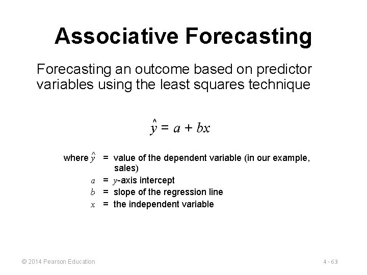
Associative Forecasting an outcome based on predictor variables using the least squares technique y^ = a + bx where y^ = value of the dependent variable (in our example, sales) a = y-axis intercept b = slope of the regression line x = the independent variable © 2014 Pearson Education 4 - 63

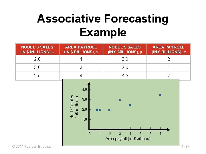
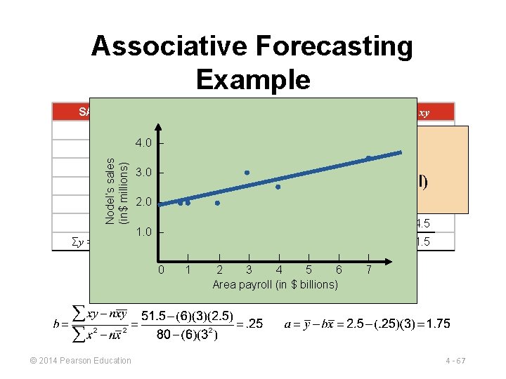
Associative Forecasting Example NODEL’S SALES (IN $ MILLIONS), y AREA PAYROLL (IN $ BILLIONS), x 2. 0 1 2. 0 2 3. 0 3 2. 0 1 2. 5 4 3. 5 7 Nodel’s sales (in$ millions) 4. 0 – 3. 0 – 2. 0 – 1. 0 – 0 | | | | 1 2 3 4 5 6 7 Area payroll (in $ billions) © 2014 Pearson Education 4 - 64

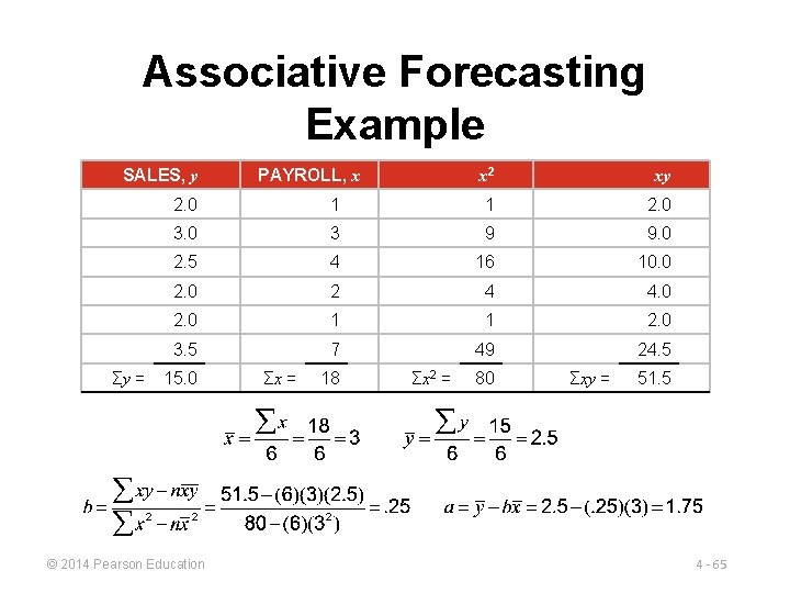
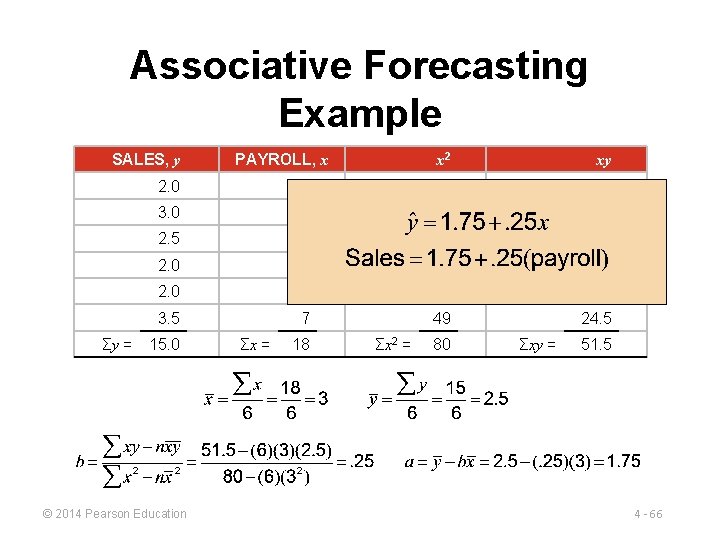
Associative Forecasting Example SALES, y PAYROLL, x x 2 xy 2. 0 1 1 2. 0 3 9 9. 0 2. 5 4 16 10. 0 2 4 4. 0 2. 0 1 1 2. 0 3. 5 7 49 24. 5 Σy = 15. 0 © 2014 Pearson Education Σx = 18 Σx 2 = 80 Σxy = 51. 5 4 - 65

Associative Forecasting Example SALES, y PAYROLL, x x 2 xy 2. 0 1 1 2. 0 3 9 9. 0 2. 5 4 16 10. 0 2 4 4. 0 2. 0 1 1 2. 0 3. 5 7 49 24. 5 Σy = 15. 0 © 2014 Pearson Education Σx = 18 Σx 2 = 80 Σxy = 51. 5 4 - 66

Associative Forecasting Example SALES, y PAYROLL, x x 2 xy 1 1 2. 0 3 9 9. 0 2. 5 3. 0 – 2. 0 – 4 16 10. 0 2 4 4. 0 1 1 2. 0 3. 5 7 49 24. 5 2. 0 4. 0 – Nodel’s sales (in$ millions) 3. 0 Σy = 15. 0 1. 0 – Σx = | 0 © 2014 Pearson Education 1 Σx 2 = 18 | | | Σxy = 80 | | | 2 3 4 5 6 Area payroll (in $ billions) 7 51. 5 4 - 67

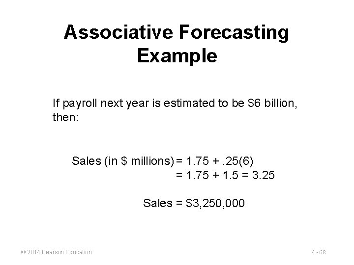
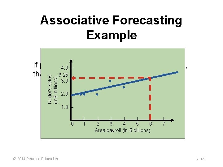
Associative Forecasting Example If payroll next year is estimated to be $6 billion, then: Sales (in $ millions) = 1. 75 +. 25(6) = 1. 75 + 1. 5 = 3. 25 Sales = $3, 250, 000 © 2014 Pearson Education 4 - 68

Associative Forecasting Example Nodel’s sales (in$ millions) If payroll 4. 0 next – year is estimated to be $6 billion, then: 3. 25 3. 0 – 2. 0 – Sales (in$ millions) = 1. 75 +. 25(6) 1. 0 – = 1. 75 + 1. 5 = 3. 25 | 0 © 2014 Pearson Education 1 | | | 2 3 4 5 6 Sales = $3, 250, 000 Area payroll (in $ billions) | 7 4 - 69

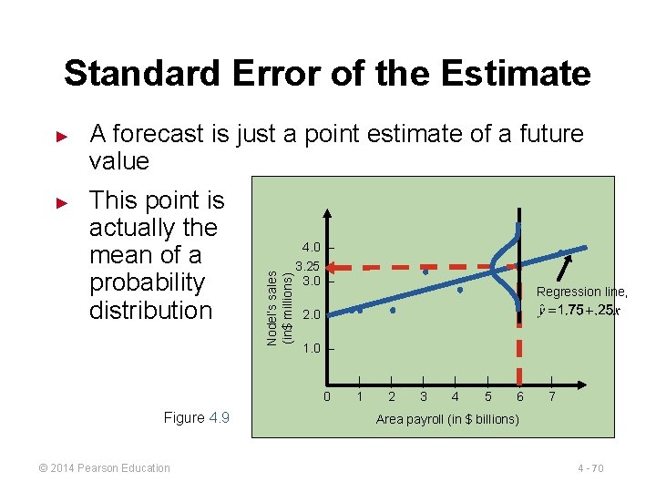
Standard Error of the Estimate ► A forecast is just a point estimate of a future value This point is actually the mean of a probability distribution Nodel’s sales (in$ millions) ► 4. 0 – 3. 25 3. 0 – 2. 0 – 1. 0 – 0 Figure 4. 9 © 2014 Pearson Education Regression line, | 1 | 2 | 3 | 4 | 5 | 6 | 7 Area payroll (in $ billions) 4 - 70

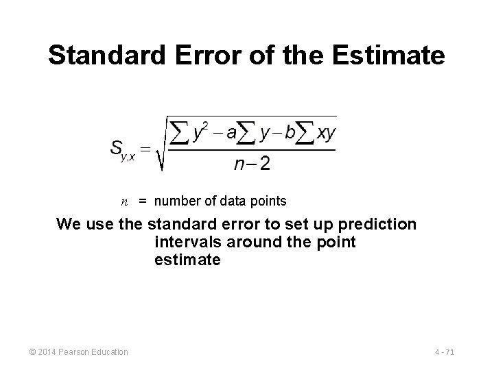
Standard Error of the Estimate n = number of data points We use the standard error to set up prediction intervals around the point estimate © 2014 Pearson Education 4 - 71

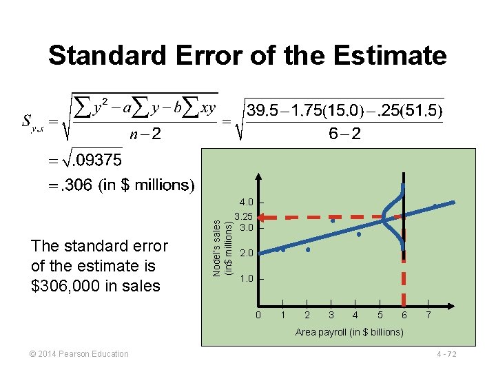
The standard error of the estimate is $306, 000 in sales Nodel’s sales (in$ millions) Standard Error of the Estimate 4. 0 – 3. 25 3. 0 – 2. 0 – 1. 0 – 0 | 1 | 2 | 3 | 4 | 5 | 6 | 7 Area payroll (in $ billions) © 2014 Pearson Education 4 - 72

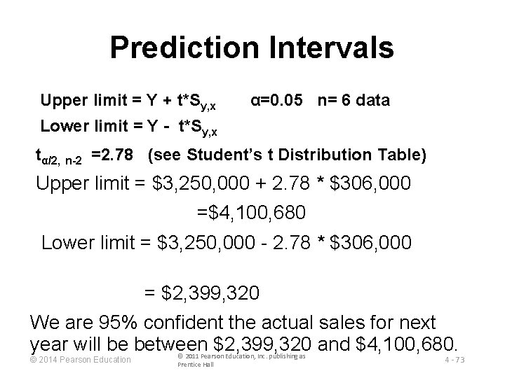
Prediction Intervals Upper limit = Y + t*Sy, x α=0. 05 n= 6 data Lower limit = Y - t*Sy, x tα/2, n-2 =2. 78 (see Student’s t Distribution Table) Upper limit = $3, 250, 000 + 2. 78 * $306, 000 =$4, 100, 680 Lower limit = $3, 250, 000 - 2. 78 * $306, 000 = $2, 399, 320 We are 95% confident the actual sales for next year will be between $2, 399, 320 and $4, 100, 680. © 2014 Pearson Education © 2011 Pearson Education, Inc. publishing as Prentice Hall 4 - 73

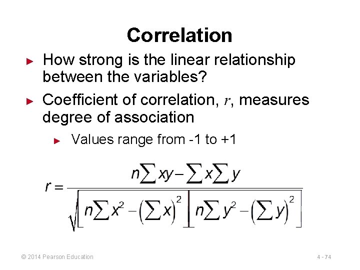
Correlation ► ► How strong is the linear relationship between the variables? Coefficient of correlation, r, measures degree of association ► Values range from -1 to +1 © 2014 Pearson Education 4 - 74

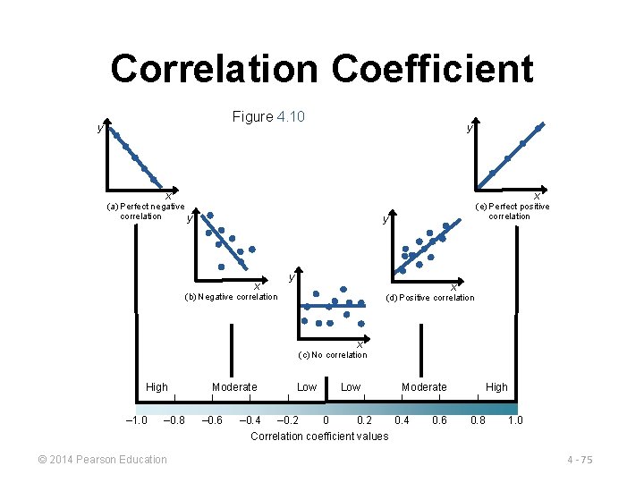
Correlation Coefficient Figure 4. 10 y y x x (a) Perfect negative correlation y (e) Perfect positive correlation y y x x (b) Negative correlation (d) Positive correlation x (c) No correlation | High – 1. 0 Moderate | | – 0. 8 – 0. 6 © 2014 Pearson Education | | Low | Moderate | – 0. 4 – 0. 2 0. 4 Correlation coefficient values | | 0. 6 0. 8 High 1. 0 4 - 75

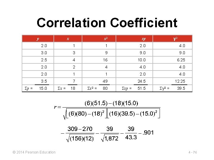
Correlation Coefficient y Σy = x x 2 xy y 2 2. 0 1 1 2. 0 4. 0 3 9 9. 0 2. 5 4 16 10. 0 6. 25 2. 0 2 4 4. 0 2. 0 1 1 2. 0 4. 0 3. 5 7 49 24. 5 12. 25 15. 0 © 2014 Pearson Education Σx = 18 Σx 2 = 80 Σxy = 51. 5 Σy 2 = 39. 5 4 - 76

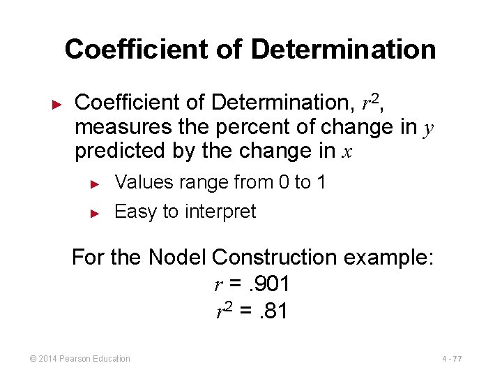
Coefficient of Determination ► Coefficient of Determination, r 2, measures the percent of change in y predicted by the change in x ► Values range from 0 to 1 ► Easy to interpret For the Nodel Construction example: r =. 901 r 2 =. 81 © 2014 Pearson Education 4 - 77

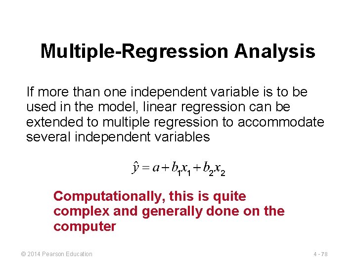
Multiple-Regression Analysis If more than one independent variable is to be used in the model, linear regression can be extended to multiple regression to accommodate several independent variables Computationally, this is quite complex and generally done on the computer © 2014 Pearson Education 4 - 78