External Costs of Poor Health ECON 40565 Fall

External Costs of Poor Health ECON 40565 Fall 2007 1

Introduction • Much of morbidity and mortality is caused by behavior – 50% of all deaths (tobacco, alcohol, driving, etc) • Sometimes these behaviors only impact the individual making the decision • Other times, the behavior can impact others – Financially – Health wise 2

Examples • Obvious examples – Infectious diseases – Drunk driving – Second hand smoke • Some not so obvious – Obesity/tobacco use increases costs of health insurance premiums for others – Your immunization reduces the chance that others will be infected 3

This section • Examine in detail general topic of externalities – Define them – Why they are ‘bad’ from an economic sense – How can we measure the size of welfare loss • Show taxes can be used to limit the social costs of an externality 4

This section • Extended example: Do smokers and drinkers pay their way? – Alcohol and cigarette consumption generates externalities – They are also taxed at the local, state and federal level – Sum up the external costs of smoking/drinking – Compare to the revenues raised by taxes – Surprising results • Excellent example of how economists look at problems 5

Before we start • Basic review of the dead weight loss from externalities • How taxes can internalize the costs of externalities 6

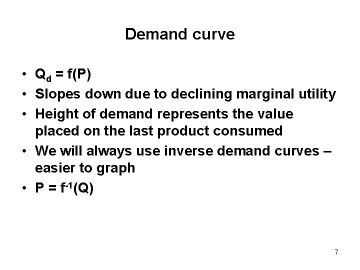
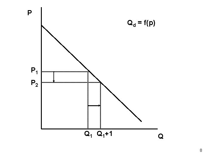
Demand curve • Qd = f(P) • Slopes down due to declining marginal utility • Height of demand represents the value placed on the last product consumed • We will always use inverse demand curves – easier to graph • P = f-1(Q) 7

P Qd = f(p) P 1 P 2 Q 1+1 Q 8

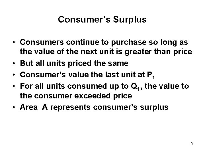
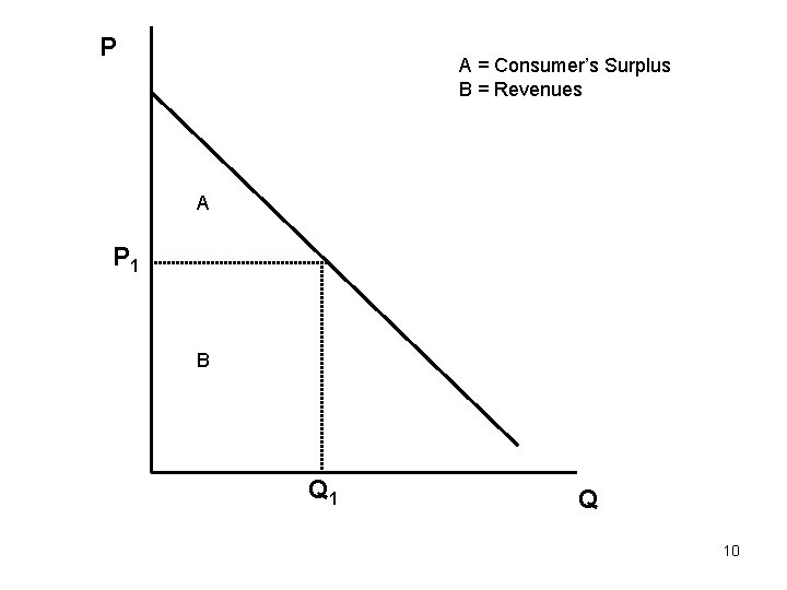
Consumer’s Surplus • Consumers continue to purchase so long as the value of the next unit is greater than price • But all units priced the same • Consumer’s value the last unit at P 1 • For all units consumed up to Q 1, the value to the consumer exceeded price • Area A represents consumer’s surplus 9

P A = Consumer’s Surplus B = Revenues A P 1 B Q 10

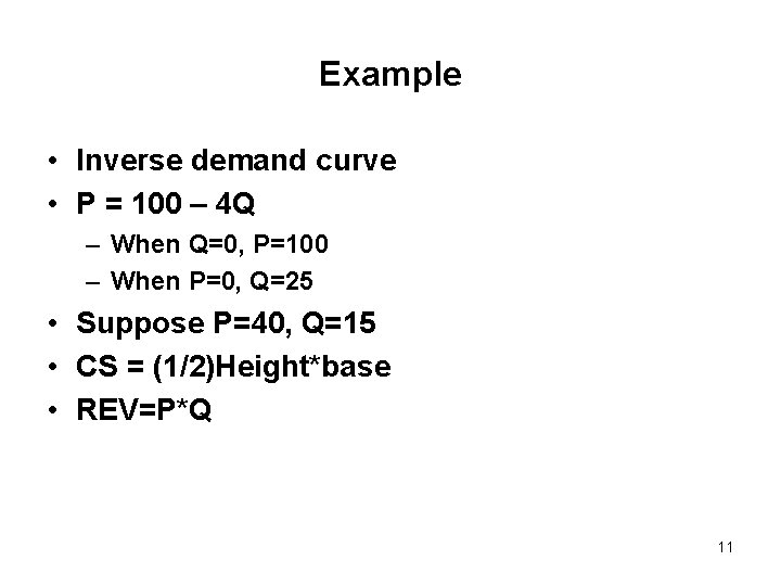
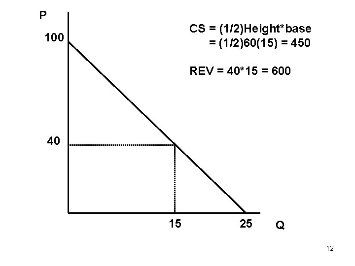
Example • Inverse demand curve • P = 100 – 4 Q – When Q=0, P=100 – When P=0, Q=25 • Suppose P=40, Q=15 • CS = (1/2)Height*base • REV=P*Q 11

P CS = (1/2)Height*base = (1/2)60(15) = 450 100 REV = 40*15 = 600 40 15 25 Q 12

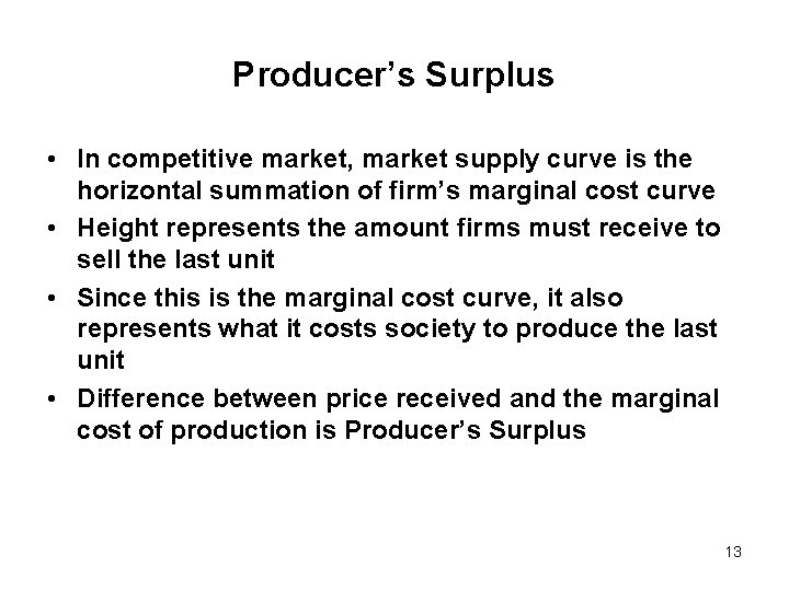
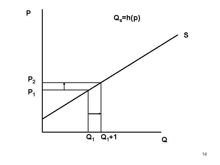
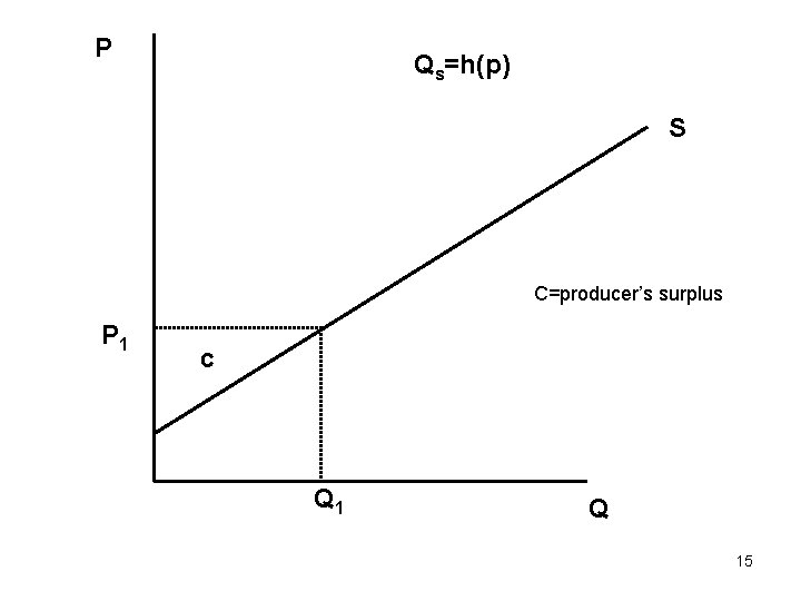
Producer’s Surplus • In competitive market, market supply curve is the horizontal summation of firm’s marginal cost curve • Height represents the amount firms must receive to sell the last unit • Since this is the marginal cost curve, it also represents what it costs society to produce the last unit • Difference between price received and the marginal cost of production is Producer’s Surplus 13

P Qs=h(p) S P 2 P 1 Q 1+1 Q 14

P Qs=h(p) S C=producer’s surplus P 1 c Q 15

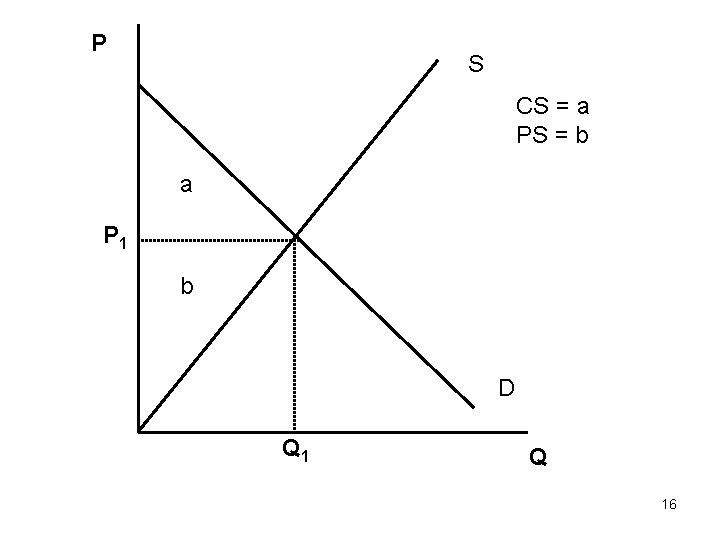
P S CS = a PS = b a P 1 b D Q 16

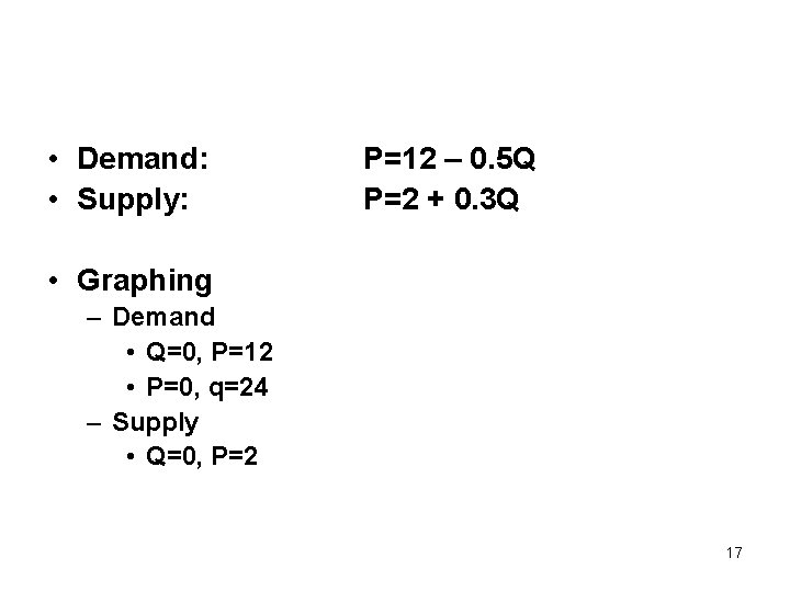
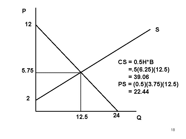
• Demand: • Supply: P=12 – 0. 5 Q P=2 + 0. 3 Q • Graphing – Demand • Q=0, P=12 • P=0, q=24 – Supply • Q=0, P=2 17

P 12 S CS = 0. 5 H*B =. 5(6. 25)(12. 5) = 39. 06 PS = (0. 5)(3. 75)(12. 5) = 22. 44 5. 75 2 12. 5 24 Q 18

Externalities • Actions of one party make another worse/better off, yet the first party does not bear all the costs/benefits • The full costs/benefits of an economic transaction are not fully captured in the transacted prices – What person pays in price – What a firm pays in costs 19

Negative Externalities • Pollution from a production process • Noise from a nightclub near a residential neighborhood • The person next to you during an exam has a cold • Second hand smoke 20

Positive Externalities • You get a flu shot. This reduces the probability others will get the flu. They benefit, you paid the costs • Your beautiful garden raises the value of your neighbor’s house • Lojak: – Transmitted on car that can be used to locate a stolen vehicle – Reduced auto thefts in areas where it was introduced – Only a small fraction had Lojak. As a result, non-Lojak users benefited 21

Excess production and negative externalities • Suppose production of the good generates externalities that are not reflected in costs of inputs (e. g. , pollution) • The true cost of producing the good is above the costs firms pay to produce • Since firms are not paying all the costs of production, the ‘wedge’ between private costs and social costs encourages overproduction 22

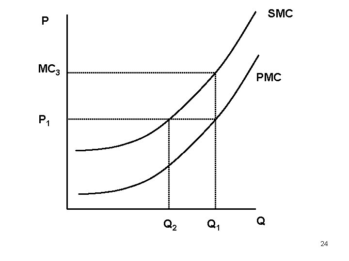
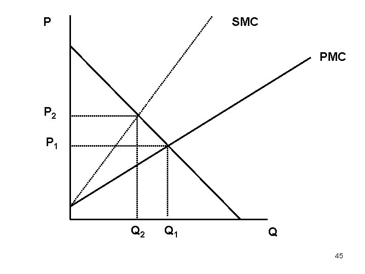
Production externalities • Perfectly competitive market. Supply Curve = marginal cost curve (MC) • Not all costs of production are borne by the firm, e. g. , pollution • PMC = private marginal cost, the firm’s costs, therefore, the industry supply • SMC = social marginal cost • SMC > PMC for all Q 23

SMC P MC 3 PMC P 1 Q 2 Q 1 Q 24

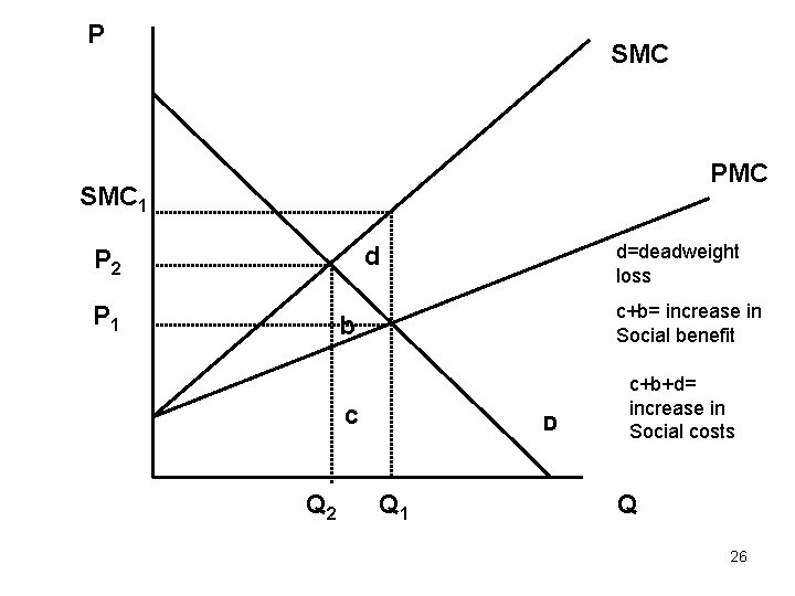
• At market price P 1, firms are willing to sell Q 1 units. However, from a social standpoint, if all costs were paid by the firm, they would only be willing to supply Q 2 • The firm overproduces the good since they do not pay all the costs of production • At Q 1, the firm receives P 1 but it costs society MC 3 to produce 25

P SMC PMC SMC 1 d=deadweight loss d P 2 P 1 c+b= increase in Social benefit b c Q 2 D Q 1 c+b+d= increase in Social costs Q 26

• Market output (P 1, Q 1) • At Q 1, SMC 1 > P 1 • Costing society more to produce than is transacted in the market • Social optimum (P 2, Q 2) 27

Social Costs of Overproduction • Notice that as one moves from Q 2 to Q 1 • Society is spending an extra d+b+c on additional resources • Consumers are however enjoying b + c in additional welfare • The difference is area d, the deadweight loss of overproduction • If there ever is a ‘wedge’ between what it costs to produce a good and what people are paying for it, there will be a deadweight loss 28

What about consumption externalities? • Standard downward sloping demand for a good • Consumption of the good however has health/financial costs to others (e. g. , second hand smoke or drunk driving) • Private Marginal Benefit > Social Marginal Benefit 29

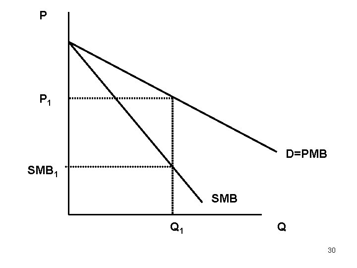
P P 1 D=PMB SMB 1 SMB Q 1 Q 30

• At Q 1, people value the last unit at P 1 • However, not all costs of the good are paid by the consumers • The SMB is SMB 1 which is lower than price • If people had to pay all the costs of the good (forget how they will do it for now), they would consume a lot less • Therefore, there is over-consumption of the good 31

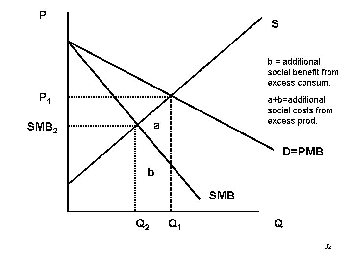
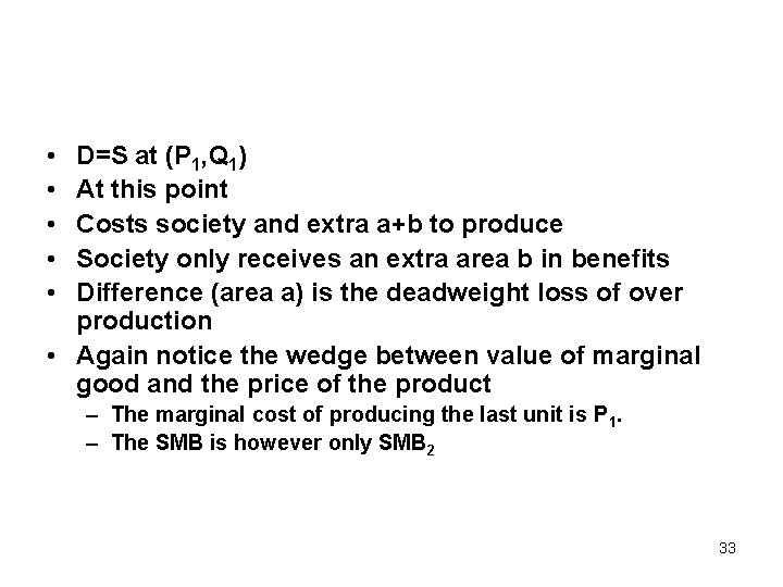
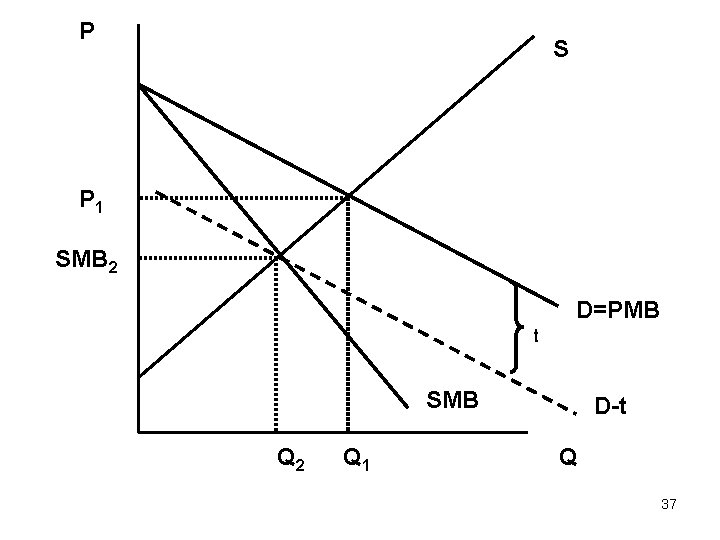
P S b = additional social benefit from excess consum. P 1 a+b=additional social costs from excess prod. a SMB 2 D=PMB b SMB Q 2 Q 1 Q 32

• • • D=S at (P 1, Q 1) At this point Costs society and extra a+b to produce Society only receives an extra area b in benefits Difference (area a) is the deadweight loss of over production • Again notice the wedge between value of marginal good and the price of the product – The marginal cost of producing the last unit is P 1. – The SMB is however only SMB 2 33

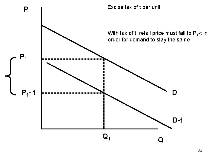
Internalize the Externality • Per unit tax on output – Pigouvian taxes • “Excise tax” • For every unit sold, charge consumers $t in a tax • The excise tax will shift down the demand curve by an amount equal to the tax • Remember, the Y (price) axis is the price transacted between buyers and sellers, does not reflect true cost 34

P Excise tax of t per unit With tax of t, retail price must fall to P 1 -t in order for demand to stay the same P 1 - t D D-t Q 1 Q 35

• Vertical axis, amount transacted between buyers and sellers • Without excise tax, at price P 1, people willing to consume Q 1 • With a tax of $t/unit, price paid to sellers would have to fall to P-t in order to demand Q 1 – Pay P 1 -t to firm – Pay t to government – Pay P 1 -t +t = P 1 in total 36

P S P 1 SMB 2 D=PMB t SMB Q 2 Q 1 D-t Q 37

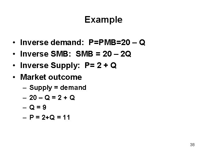
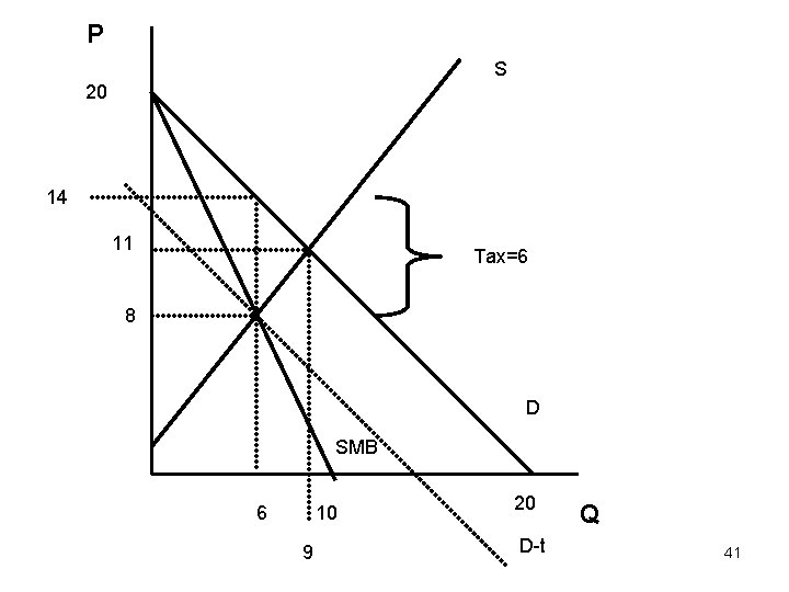
Example • • Inverse demand: P=PMB=20 – Q Inverse SMB: SMB = 20 – 2 Q Inverse Supply: P= 2 + Q Market outcome – – Supply = demand 20 – Q = 2 + Q Q=9 P = 2+Q = 11 38

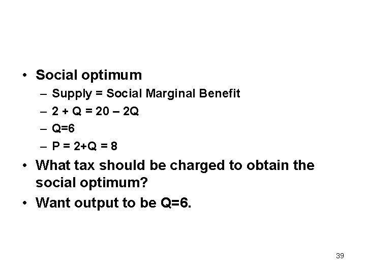
• Social optimum – – Supply = Social Marginal Benefit 2 + Q = 20 – 2 Q Q=6 P = 2+Q = 8 • What tax should be charged to obtain the social optimum? • Want output to be Q=6. 39

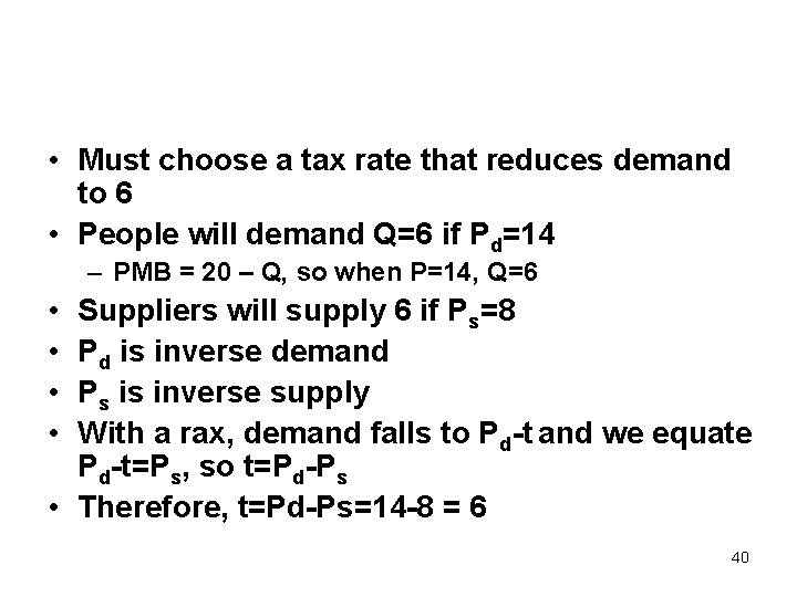
• Must choose a tax rate that reduces demand to 6 • People will demand Q=6 if Pd=14 – PMB = 20 – Q, so when P=14, Q=6 • • Suppliers will supply 6 if Ps=8 Pd is inverse demand Ps is inverse supply With a rax, demand falls to Pd-t and we equate Pd-t=Ps, so t=Pd-Ps • Therefore, t=Pd-Ps=14 -8 = 6 40

P S 20 14 11 Tax=6 8 D SMB 6 10 9 20 D-t Q 41

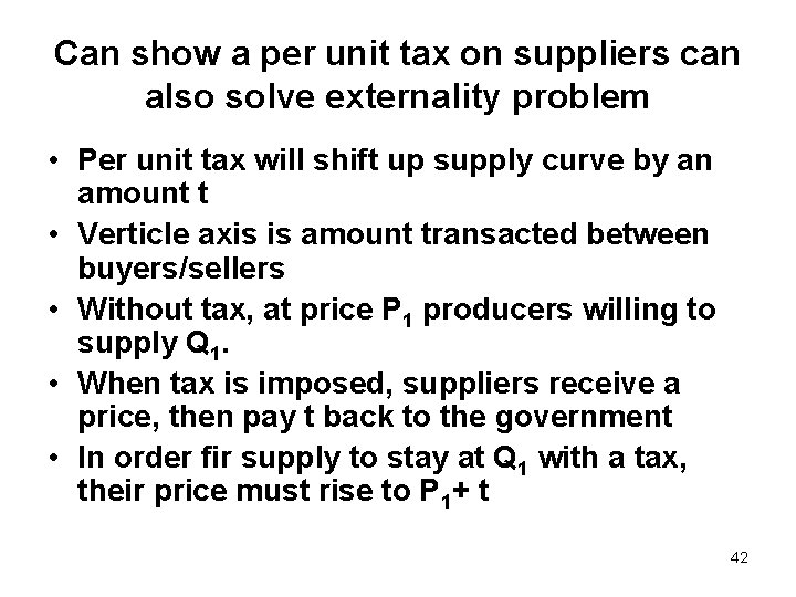
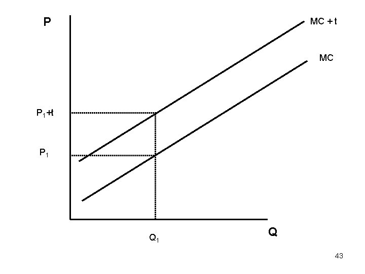
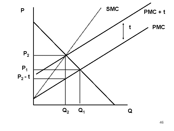
Can show a per unit tax on suppliers can also solve externality problem • Per unit tax will shift up supply curve by an amount t • Verticle axis is amount transacted between buyers/sellers • Without tax, at price P 1 producers willing to supply Q 1. • When tax is imposed, suppliers receive a price, then pay t back to the government • In order fir supply to stay at Q 1 with a tax, their price must rise to P 1+ t 42

P MC + t MC P 1+t P 1 Q 43

• At P 1, firms were willing to supply Q 1 • With an excise tax, in order for firms to supply Q 1, the price must increase to P 1+t – Firm receives P 1+t – Pay the government t in taxes – Net P 1 • Therefore, an excise tax will shift the supply curve up by the amount of the tax 44

P SMC P 2 P 1 Q 2 Q 1 Q 45

SMC P PMC + t t PMC P 2 P 1 P 2 - t Q 2 Q 1 Q 46

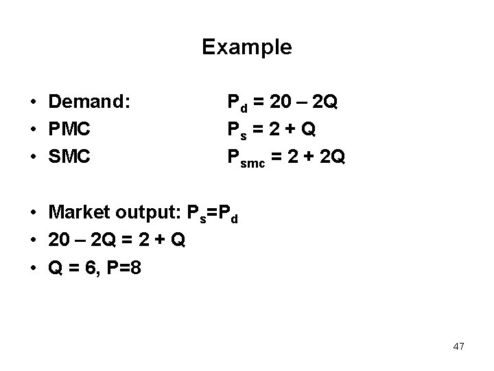
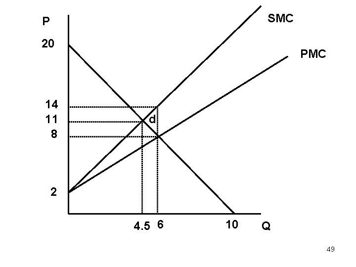
Example • Demand: • PMC • SMC Pd = 20 – 2 Q Ps = 2 + Q Psmc = 2 + 2 Q • Market output: Ps=Pd • 20 – 2 Q = 2 + Q • Q = 6, P=8 47

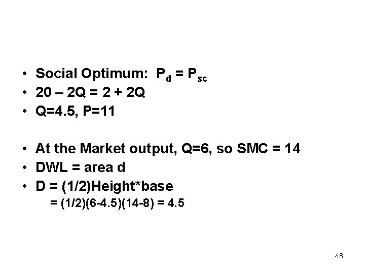
• Social Optimum: Pd = Psc • 20 – 2 Q = 2 + 2 Q • Q=4. 5, P=11 • At the Market output, Q=6, so SMC = 14 • DWL = area d • D = (1/2)Height*base = (1/2)(6 -4. 5)(14 -8) = 4. 5 48

SMC P 20 14 11 8 PMC d 2 4. 5 6 10 Q 49

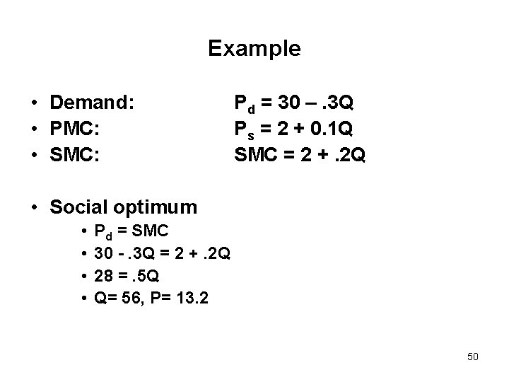
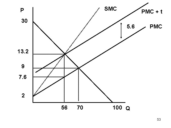
Example • Demand: • PMC: • SMC: Pd = 30 –. 3 Q Ps = 2 + 0. 1 Q SMC = 2 +. 2 Q • Social optimum • • Pd = SMC 30 -. 3 Q = 2 +. 2 Q 28 =. 5 Q Q= 56, P= 13. 2 50

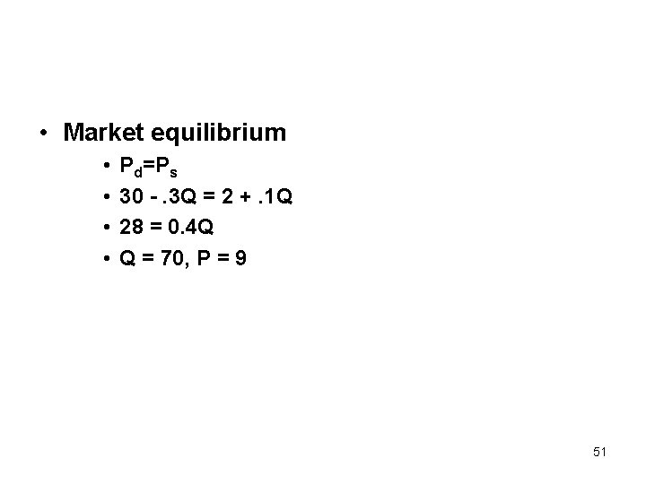
• Market equilibrium • • Pd=Ps 30 -. 3 Q = 2 +. 1 Q 28 = 0. 4 Q Q = 70, P = 9 51

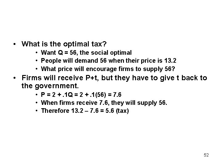
• What is the optimal tax? • Want Q = 56, the social optimal • People will demand 56 when their price is 13. 2 • What price will encourage firms to supply 56? • Firms will receive P+t, but they have to give t back to the government. • P = 2 +. 1 Q = 2 +. 1(56) = 7. 6 • When firms receive 7. 6, they will supply 56. • Therefore 13. 2 – 7. 6 = 5. 6 (tax) 52

SMC P 30 PMC + t 5. 6 PMC 13. 2 9 7. 6 2 56 70 100 Q 53

Excises taxes on poor health • Alcohol and cigarettes are taxed at the federal, state and local level • Some states sell liquor rather than tax it (VA, PA, etc. ) • Most of these taxes are excise taxes -- the tax is per unit – Rates differ by type of alcohol, alcohol content – Nearly all cigarettes taxed the same 54

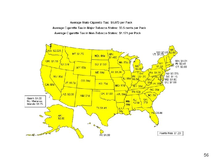
Current excise tax rates • http: //www. taxfoundation. org/publications/sh ow/245. html • Cigarettes – Low: KY ($0. 30/pack), VA ($0. 30), SC($0. 07) – High: RI ($2. 46), NJ ($2. 58) – Average of $1. 07 across states • Beer – Low (WY, $0. 02/gallon) – High (SC, $0. 77/gallon) 55

56

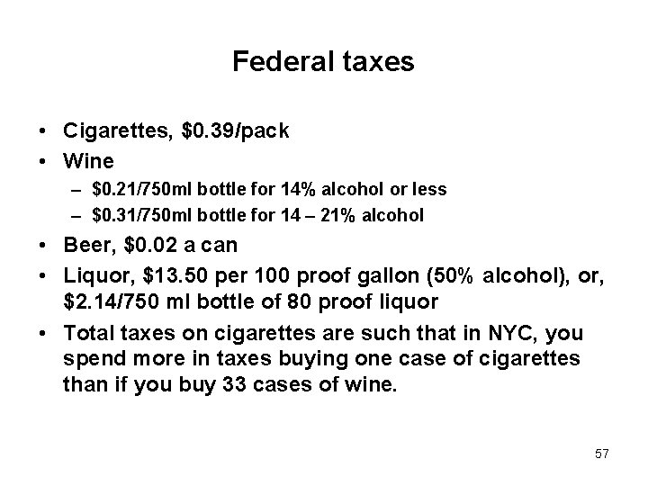
Federal taxes • Cigarettes, $0. 39/pack • Wine – $0. 21/750 ml bottle for 14% alcohol or less – $0. 31/750 ml bottle for 14 – 21% alcohol • Beer, $0. 02 a can • Liquor, $13. 50 per 100 proof gallon (50% alcohol), or, $2. 14/750 ml bottle of 80 proof liquor • Total taxes on cigarettes are such that in NYC, you spend more in taxes buying one case of cigarettes than if you buy 33 cases of wine. 57

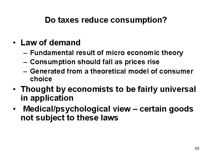
Do taxes reduce consumption? • Law of demand – Fundamental result of micro economic theory – Consumption should fall as prices rise – Generated from a theoretical model of consumer choice • Thought by economists to be fairly universal in application • Medical/psychological view – certain goods not subject to these laws 58

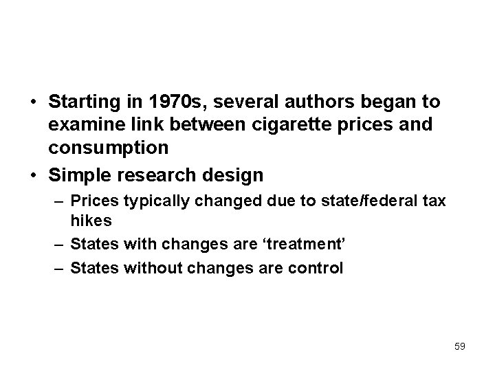
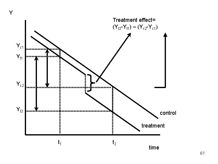
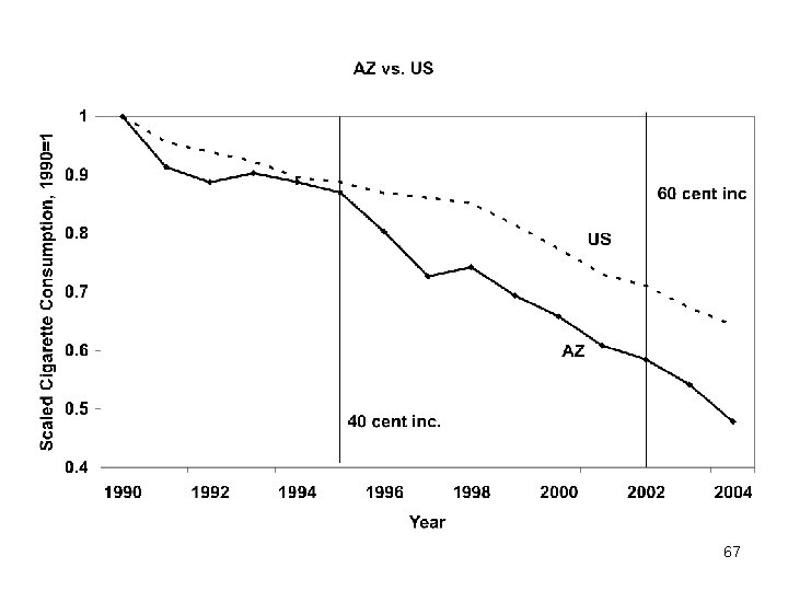
• Starting in 1970 s, several authors began to examine link between cigarette prices and consumption • Simple research design – Prices typically changed due to state/federal tax hikes – States with changes are ‘treatment’ – States without changes are control 59

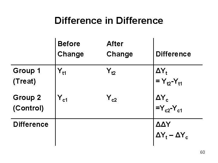
Difference in Difference Before Change After Change Group 1 (Treat) Yt 1 Yt 2 ΔYt = Yt 2 -Yt 1 Group 2 (Control) Yc 1 Yc 2 ΔYc =Yc 2 -Yc 1 Difference ΔΔY ΔYt – ΔYc 60

Y Treatment effect= (Yt 2 -Yt 1) – (Yc 2 -Yc 1) Yc 1 Yt 1 Yc 2 Yt 2 control treatment t 1 t 2 time 61

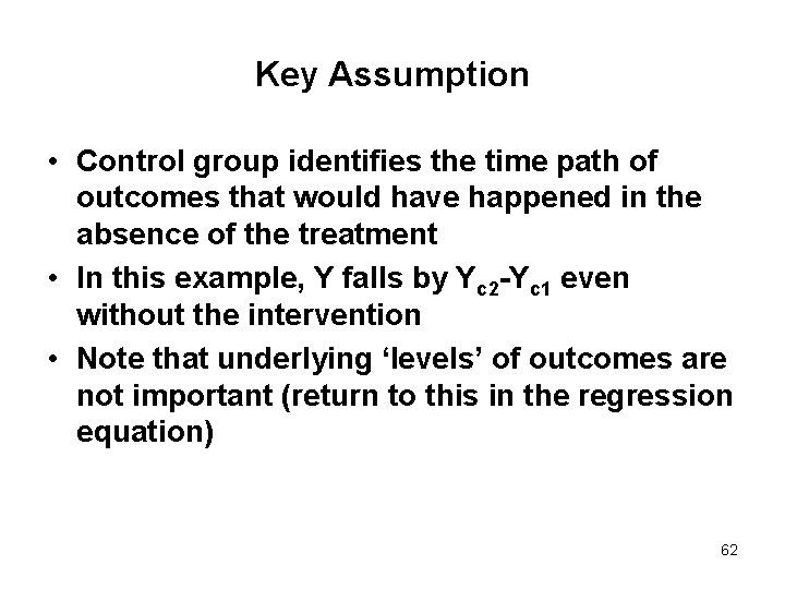
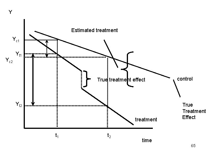
Key Assumption • Control group identifies the time path of outcomes that would have happened in the absence of the treatment • In this example, Y falls by Yc 2 -Yc 1 even without the intervention • Note that underlying ‘levels’ of outcomes are not important (return to this in the regression equation) 62

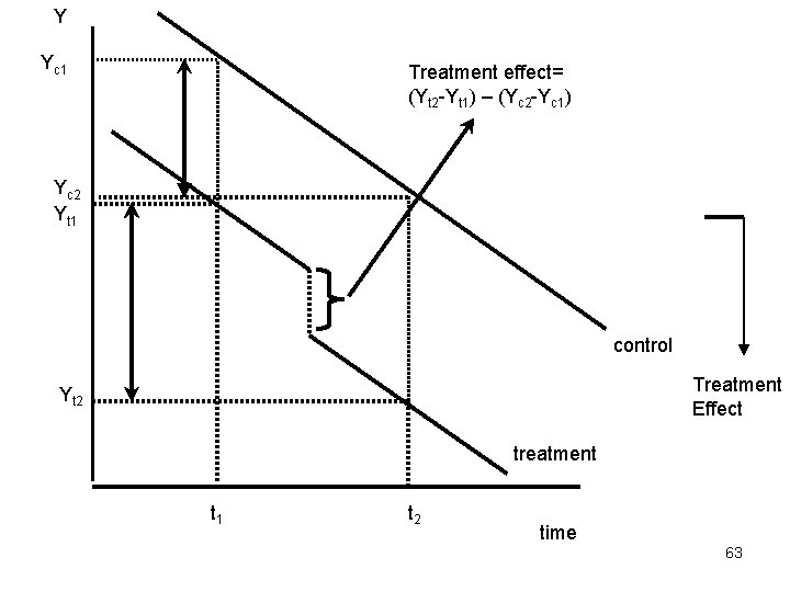
Y Yc 1 Treatment effect= (Yt 2 -Yt 1) – (Yc 2 -Yc 1) Yc 2 Yt 1 control Treatment Effect Yt 2 treatment t 1 t 2 time 63

• In contrast, what is key is that the time trends in the absence of the intervention are the same in both groups • If the intervention occurs in an area with a different trend, will under/over state the treatment effect • In this example, suppose intervention occurs in area with faster falling Y 64

Y Estimated treatment Yc 1 Yc 2 Yt 1 True treatment effect Yt 2 treatment t 1 t 2 control True Treatment Effect time 65

• Near universal agreement in results – 10% increase in price reduces demand by 4% – Change in smoking evenly split between • Reductions in number of smokers • Reductions in cigs/day among remaining smokers • Results have been replicated – in other countries/time periods, variety of statistical models, subgroups – For other addictive goods: alcohol, cocaine, marijuana, heroin, gambling 66

67

68

69

70

Taxes now an integral part of antismoking campaigns • Key component of ‘Master Settlement’ • Surgeon General’s report – “raising tobacco excise taxes is widely regarded as one of the most effective tobacco prevention and control strategies. ” • Tax hikes are now designed to reduce smoking 71

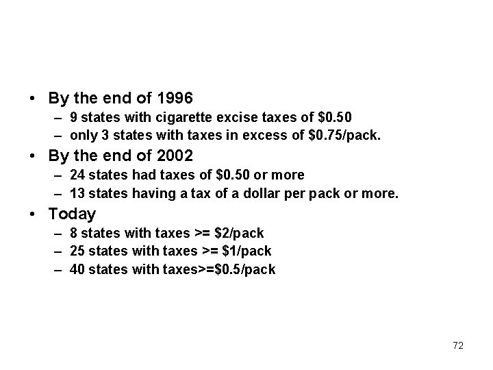
• By the end of 1996 – 9 states with cigarette excise taxes of $0. 50 – only 3 states with taxes in excess of $0. 75/pack. • By the end of 2002 – 24 states had taxes of $0. 50 or more – 13 states having a tax of a dollar per pack or more. • Today – 8 states with taxes >= $2/pack – 25 states with taxes >= $1/pack – 40 states with taxes>=$0. 5/pack 72

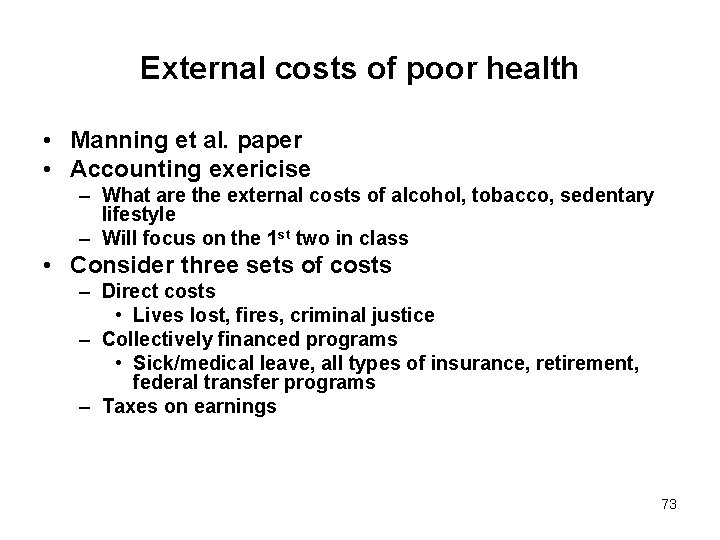
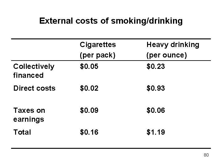
External costs of poor health • Manning et al. paper • Accounting exericise – What are the external costs of alcohol, tobacco, sedentary lifestyle – Will focus on the 1 st two in class • Consider three sets of costs – Direct costs • Lives lost, fires, criminal justice – Collectively financed programs • Sick/medical leave, all types of insurance, retirement, federal transfer programs – Taxes on earnings 73

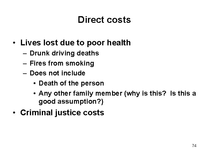
Direct costs • Lives lost due to poor health – Drunk driving deaths – Fires from smoking – Does not include • Death of the person • Any other family member (why is this? Is this a good assumption? ) • Criminal justice costs 74

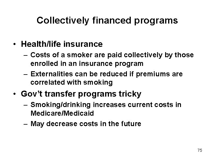
Collectively financed programs • Health/life insurance – Costs of a smoker are paid collectively by those enrolled in an insurance program – Externalities can be reduced if premiums are correlated with smoking • Gov’t transfer programs tricky – Smoking/drinking increases current costs in Medicare/Medicaid – May decrease costs in the future 75

Taxes on Earnings • Smokers and heavy drinkers – Are less productive during working years (do not know whether this is causal) – If die prematurely, pay less in state/local income taxes 76

What is NOT an external cost • The smoker/drinkers diminished health or the health of their family members • The lost earnings of these activities • Why? 77

Special case of Federal Programs • Expenditures are correlated with longevity – Social security, Medicare/Medicaid costs increase for older people • Because smoking kills people early – Prevents people from getting to the age when medical costs are very high – Reduces payment of Social Security benefits 78

• From the perspective of the other taxpayers, these are positive externalities • Smokers pay $ to Federal and states • They do not take as much out (SS, Medicare/caid) because they die early 79

External costs of smoking/drinking Cigarettes (per pack) Heavy drinking (per ounce) Collectively financed $0. 05 $0. 23 Direct costs $0. 02 $0. 93 Taxes on earnings $0. 09 $0. 06 Total $0. 16 $1. 19 80

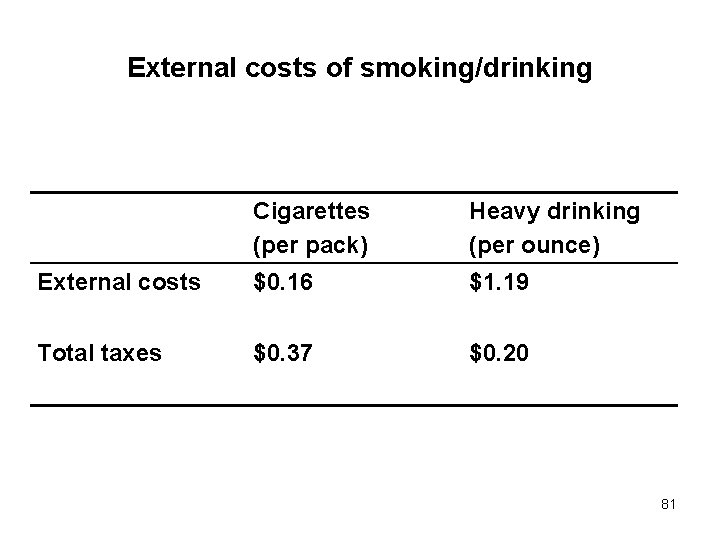
External costs of smoking/drinking Cigarettes (per pack) Heavy drinking (per ounce) External costs $0. 16 $1. 19 Total taxes $0. 37 $0. 20 81

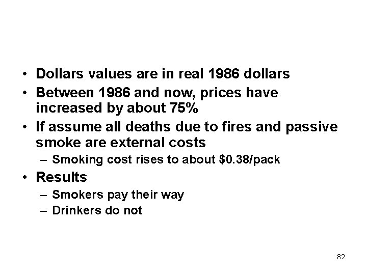
• Dollars values are in real 1986 dollars • Between 1986 and now, prices have increased by about 75% • If assume all deaths due to fires and passive smoke are external costs – Smoking cost rises to about $0. 38/pack • Results – Smokers pay their way – Drinkers do not 82

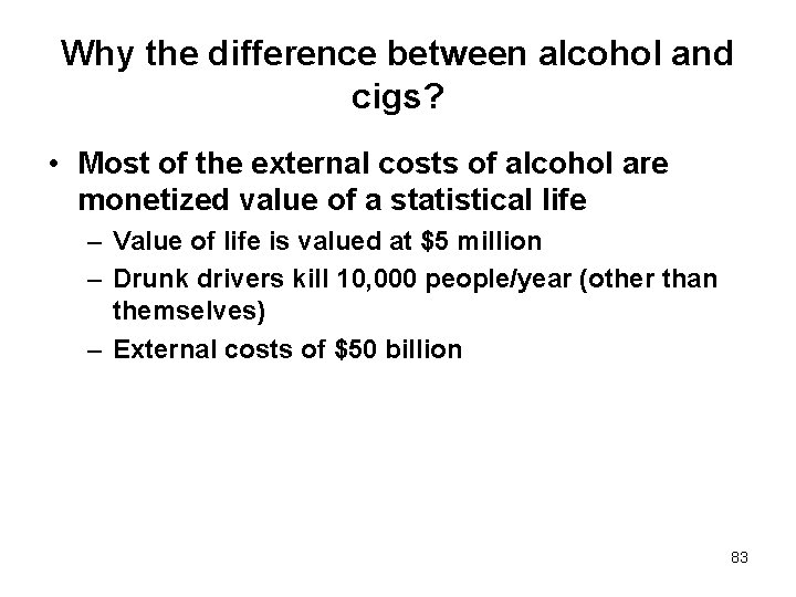
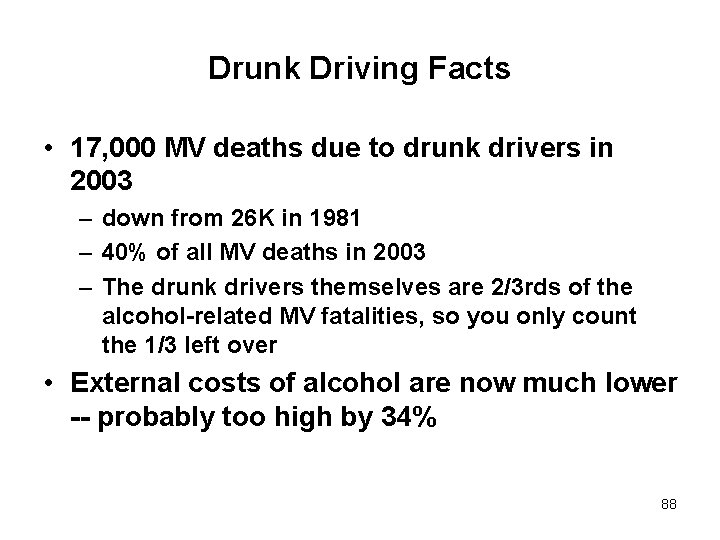
Why the difference between alcohol and cigs? • Most of the external costs of alcohol are monetized value of a statistical life – Value of life is valued at $5 million – Drunk drivers kill 10, 000 people/year (other than themselves) – External costs of $50 billion 83

Value of a statistical life • People trade off $ for job characteristics – Jobs with nice characteristics paid less – Jobs with unattractive characteristics paid more – Hold ALL ELSE CONSTANT • One characteristic is job risk • Workers in higher risk jobs get paid more • Can use the willingness to accept risk to calculate a ‘statistical value of life’ 84

• Among blue collar workers, there is a 1 in 10, 000 chance of dying on the job during the year. • People in jobs with twice the average risk are estimated to make $500 more than identical people in average risk jobs. • For every additional 10, 000 workers in highrisk jobs, they will receive and extra $500 x 10, 000 = $5 million in income 85

• But among these additional workers, on average, 1 will die. • VSL=value of a statistical life • VSL = additional income people are willing to take for additional risk/expected additional deaths 86

• Example: Suppose that a group of workers requires an additional $350 to accept an additional risk of death of 0. 000152 • Just divide $350/0. 000152 = $2. 3 million • Suppose there an addition 50000 workers – Take home an additional 50000*350 = $17. 5 million – But an additional 50000*0. 000152 = 7. 6 will die – 17. 5/7. 6=$2. 3 million 87

Drunk Driving Facts • 17, 000 MV deaths due to drunk drivers in 2003 – down from 26 K in 1981 – 40% of all MV deaths in 2003 – The drunk drivers themselves are 2/3 rds of the alcohol-related MV fatalities, so you only count the 1/3 left over • External costs of alcohol are now much lower -- probably too high by 34% 88

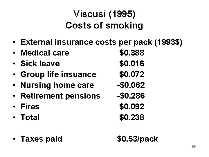
Viscusi (1995) Costs of smoking • • External insurance costs per pack (1993$) Medical care $0. 388 Sick leave $0. 016 Group life insuance $0. 072 Nursing home care -$0. 062 Retirement pensions -$0. 286 Fires $0. 092 Total $0. 238 • Taxes paid $0. 53/pack 89

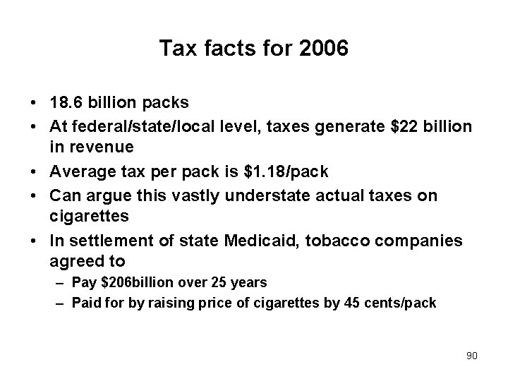
Tax facts for 2006 • 18. 6 billion packs • At federal/state/local level, taxes generate $22 billion in revenue • Average tax per pack is $1. 18/pack • Can argue this vastly understate actual taxes on cigarettes • In settlement of state Medicaid, tobacco companies agreed to – Pay $206 billion over 25 years – Paid for by raising price of cigarettes by 45 cents/pack 90

What is not included in these numbers? • Second hand smoked deaths – Disagreement about extent of deaths – Most exposure is within house – Is this an externality • Costs to children – Increases miscarriages – Increases LBW 91

What are some other justifications for higher cigarette taxes • Recall the market graph. The problem w/ external costs is that people consume above a socially optimal level • Can be other reasons why people ‘over consumer’ smoking • Maybe people do not understand the health risks. If they did, they would not smoke 92

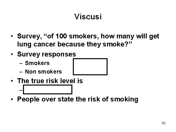
Viscusi • Survey, “of 100 smokers, how many will get lung cancer because they smoke? ” • Survey responses – Smokers – Non smokers 37/100 43/100 • The true risk level is – 5 to 10 per 100 • People over state the risk of smoking 93

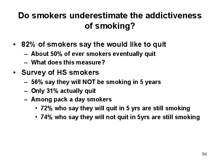
Do smokers underestimate the addictiveness of smoking? • 82% of smokers say the would like to quit – About 50% of ever smokers eventually quit – What does this measure? • Survey of HS smokers – 56% say they will NOT be smoking in 5 years – Only 31% actually quit – Among pack a day smokers • 72% who say they will quit in 5 yrs are still smoking • 74% who say they will not quit in 5 yrs are still smoking 94