Week 6 Economics Topics of Week 6 1

Week #6 Economics

Topics of Week #6 1. 2. 3. 4. 5. 6. 7. 8. Explicit Cost Implicit Cost Accounting Profit Economic Profit Short-Run vs. Long-Run* TP, MP, AP, and DMP* TC, TVC, and TFC ATC, AVC, and AFC* "*" Indicates the most important topics. Mateer ve Coppock: Chapter #8

Calculating Profit and Loss • Total Revenue (TR) – The amount a firm receives from the sale of goods and services. • Total Cost (TC) – The amount a firm spends in order to produce those goods and services. Profit (or loss) = TR – TC – Profits occurs when TR > TC – Losses occurs when TR < TC

Explicit and Implicit Costs • Explicit costs – Tangible expenses: Bills that the owner has to pay. – Wages, insurance, and food ingredients. • Implicit costs – Opportunity costs of doing business. – Opportunity cost of capital. • Bought a franchise for a large sum of money. How could the money have been invested otherwise? – Opportunity cost of owner's time above salary paid. • How much could the owner get paid elsewhere?

Explicit and Implicit Costs Explicit Costs Implicit Costs The electricity bill Labor of owner who works for the company but does not draw a salary Advertising in the newspaper The capital invested in the business Employee wages The use of the owner's car, computer, or other personal equipment to conduct business

Profits • Accounting Profit – Does not take into account implicit costs of doing business. Accounting Profit = Total Revenues – Explicit Costs • Economic Profit – Considers "All Costs" = Explicit Costs + Implicit Costs Economic Profit = Total Revenues – All Costs *As Economists, we use "All Costs" and define it as Total Cost. Similarly, we use "Economic Profit" in our analyses. In short we call it "Profit".

Rates of Return, Historically

Accounting and Economic Profits Item Cost Type Revenues Amount ($) $8, 000 Workers' Wages Explicit $4, 000 Insurance and Rent Explicit $2, 500 Food Ingredients Explicit $1, 000 Accounting Profits $8, 000 - $7, 500 = $500 Opportunity Cost of Owner's Time Implicit $300 Opportunity Cost of Owner's Capital Implicit $400 Economic Profits $8, 000 - $8, 200 = -$200

Production • Input – Resources used in the production process. Also called factors of production. – Labor (L), Capital (K), and sometimes materials (M). • Output – The product that the firm creates: Input: Capital (K) Labor (L) The firm's production process Output (Q)

Production Function • Production function – The relationship between inputs and outputs. – To create output, the owner needs to decide how many inputs to employ. • Mathematically: Q = f (K, L)

Short-Run vs. Long-Run – Short-Run: is a period of production during which some inputs cannot be varied. – Long-Run: is a period of production during which all inputs can vary. In the long-run there are no fixed inputs. – Variable Input: is one whose quantity can be changed over the short-run. – Fixed Input: is one whose quantity cannot be changed over the short-run. – We will assume labor is a variable input and capital is a fixed input in the short-run.

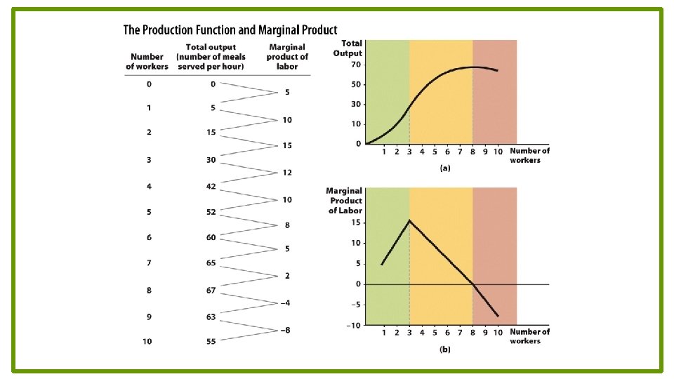
Total Product • Total Product: – Describes how output varies in the short-run as more of any one input is used together with fixed amounts of other inputs. – Total Product (TP) : Q • Total Product of Labor: – The amount of output produced over a given period by a certain amount of labor (L) employed together with fixed inputs (K). – Total Product of Labor: TPL

Marginal Product • Marginal Product (MP) of an input is the increase in output from one more unit of that input when the quantity of all other inputs is unchanged. – Change in output divided by the change in input. – Marginal Product of Labor (MPL) – Marginal Product of Capital (MPK) • Mathematically:

Marginal Product of Labor • Marginal Product of Labor (MPL) – The extra output produced with one more unit of labor. • MPL increases at first and then decreases. – When MPL is decreasing, the rate of increase in total product (TP) is declining since MPL is the slope of the TP curve. – When the marginal product of labor is zero, total product is at its maximum value. – When the marginal product is negative, additional workers decrease the total product. • Mathematically:

The Law of Diminishing Marginal Product • The extra production obtained from increases in a variable input will eventually decrease as more of the variable input is used together with the fixed inputs. • Diminishing Marginal Product (DMP) – Successive increases in an input eventually cause output to increase at a slower rate. – The point of diminishing returns corresponds to the level that the marginal product begins to decline.

The Law of Diminishing Marginal Product • Assuming capital (K) is fixed, we eventually get to a point where a new worker (L) adds less output than the previous worker. • Example: • Laborer #3 increases output by 15. • Laborer #4 increases output by 12. • Laborer #5 increases output by 10.

Why Does This Happen? • Think about the fixed amount of capital: – "Too many cooks in the kitchen". – Extra workers will eventually have less work to do, won't be able to add as much to the overall output. – Not because new workers are less skilled. • With a very large amount of L: – New workers could actually interfere with existing workers and slow them down. – This means negative marginal product!

Illustration of Diminishing MPL • Use garbage collection as an example: • Fixed input – Capital – One truck • Variable input – Labor – Workers on the truck • Output – Trash cans picked up

Average Product • The average product of an input is the total output produced over a given period divided by the number of units of that input used. – The notation we use is AP.

Average Product of Labor • The average product of labor (APL)is output per unit labor. • The APL is a measure of productivity. • The APL increases at first, reaches a maximum, and then decreases. So, the labor productivity increases at first and then decreases. • Although APL becomes smaller and smaller, it never reaches to zero.

Average Product of Labor

Margin and Average Relationship • How do we know if the average product will increase or decrease when we produce more? – We need to compare the current average to the marginal product of producing another unit. • Key phrase to remember: – "The average follows the margin. " • If the margin is above the average – The average will increase. • If the margin is below the average – The average will decrease.

Margin and Average Relationship • Suppose Lebron James has a scoring average of 30 points per game. – If he has a game in which he scores 45 points • His average increases. – If he has a game in which he scores 12 points • His average decreases. • Once again: – The average follows the margin

MPL and APL Relationship • When MPL > APL the average product of labor will rise. • When MPL = APL the average product of labor will be at the maximum. • When MPL < APL the average product of labor will decline. • DMPL implies that the average product of labor will eventually decline as more of labor is used together with fixed inputs. • Law of diminishing marginal returns decline in MPL • Decline in MPL eventually causes decline in APL

Economics in Seinfeld • "Seinfeld" – An introduction to costs. – Changing the cost structure by lowering costs can make an activity more profitable.

Costs in the Short-Run • Variable Costs (VC) – Costs that are directly related with the rate of output. – Worker wages, electric bill, and food ingredients. • Fixed Costs (FC) – – Costs that do not vary with output. Costs that exist even if output is zero. Building rent, insurance, and down-payments. Costs that must be incurred in the short-run even if the firm does not produce anything. There is no fixed cost in long-run. • Total Costs (TC) – The sum of variable and fixed costs.

Costs in the Short-Run • Average Total Cost (ATC) – Total cost divided by the number of units produced: "cost per unit. " • Analogously, – Average Variable Cost (AVC) – Average Fixed Cost (AFC) • Marginal Cost (MC) – The increase in total cost that occurs from producing additional output. – Change in total cost divided by change in output.

Some Notes About the Equations • MC Set ΔQ = 1 – Easy if we can set the denominator equal to 1 – Makes division and intuition simpler. • AFC – Will always decrease as we produce more output. – Why?

Cost Equations

TFC TC AVC TVC + TFC TVC ÷ Q ATC TC ÷ Q AFC MC TFC ÷ Q Δ TVC÷ΔQ or AVC + AFC Q TVC 0 $0. 00 $100. 00 10 30. 00 100. 00 130. 00 $3. 00 $10. 00 $13. 00 $3. 00 20 50. 00 100. 00 150. 00 2. 50 5. 00 7. 50 2. 00 30 65. 00 100. 00 165. 00 2. 17 3. 33 5. 50 1. 50 40 77. 00 100. 00 177. 00 1. 93 2. 50 4. 43 1. 20 50 87. 00 100. 00 187. 00 1. 74 2. 00 3. 74 1. 00 60 100. 00 200. 00 1. 67 3. 34 1. 30 70 120. 00 100. 00 220. 00 1. 71 1. 43 3. 14 2. 00 80 160. 00 100. 00 260. 00 2. 00 1. 25 3. 25 4. 00 90 220. 00 100. 00 320. 00 2. 44 1. 11 3. 55 6. 00 100 300. 00 100. 00 400. 00 3. 00 1. 00 4. 00 8. 00

Practice What You Know Using the Equations • Fill in the table below using the cost equations. • You have five minutes. Work with your classmates! Q TVC TFC 0 1 7 2 3 4 TC AVC AFC ATC MC 720 -- -- 740 15 202

Practice What You Know Using the Equations • Fill in the table below using the cost equations. Q TVC TFC TC AVC AFC ATC MC 0 0 720 -- -- 1 7 720 727 7 2 20 740 10 360 370 13 3 45 720 765 15 240 255 25 4 88 720 808 22 180 202 43

TC, TVC, and TFC

MC, ATC, AVC, and AFC

Why U-Shaped Cost Curves? • Why are the short-run cost curves, including the ATC, AVC, and MC, U-shaped? – Diminishing marginal product! • Explanation? – Assume all labor is paid the same wage. – Eventually, inputs become less productive at the margin (lower productivity). – This implies that output costs will start to rise.

Why U-Shaped Cost Curves? • Is there a mathematical relationship between input productivity and output costs? • Example – Each worker gets paid w = $100. – If Bob has high MPL and produces q = 20, the cost of those output units is $5 each. – If Carl has low MPL and produces q = 10, the cost of those output units is $10 each.

Economics in The Office • "The Office, Broke" – Michael Scott starts his own paper company to compete with Staples and Dunder Mifflin.

Economics in The Simpsons • "The Simpsons" – "Homer Versus Lisa & the 8 th Commandment" – Variable costs and fixed costs

Conclusion • Costs are defined in a number of ways, but marginal cost plays the most crucial role in a firm's cost structure. • By observing what happens to marginal cost you can understand changes in average cost and total cost. This is why economists place so much emphasis on marginal costs.

Summary • Economists break cost into two components. – Explicit costs (can be easily calculated). – Implicit costs (are hard to calculate). • There also two types of profits. – Accounting profits • Occurs when revenues are larger than the explicit costs. – Economic profits • Occurs when revenues are larger than the combination of explicit and implicit costs. • To optimize production, firms must effectively combine labor and capital in the right quantities.

Summary • In any short-run production process there will be a point of diminishing marginal product. – Adding additional units of a variable input will no longer produce as much additional output as before.

Summary • The MC curve always leads the ATC and AVC curves. • With the exception of the AFC curve, which always declines, short-run cost curves are U-shaped. – All variable costs initially decline due to increased specialization. – Eventually, the advantages of continued specialization give way to diminishing marginal product and the MC, AVC, and ATC curves begin to rise.

Practice What You Know Bob runs a small family restaurant. How would you describe the monthly rent he pays on the building? A. B. C. D. Explicit cost, variable cost. Explicit cost, fixed cost. Implicit cost, variable cost. Implicit cost, fixed cost.

Practice What You Know Which of the following is an example of an implicit cost? A. B. C. D. Wages paid to employees. Cost of food delivery. The opportunity cost of the owner's time. Monthly insurance premiums.

Practice What You Know Assuming the existence of efficient scale, the MC, ATC, and AVC curves are: A. B. C. D. Vertical Horizontal hill-shaped U-shaped

Practice What You Know Suppose the wage rate that a company pays its workers increases. In terms of the cost equations, which of the following is true? A. B. C. D. TC will increase, but ATC will decrease. TVC will increase, but AVC will decrease. The MC curve will become hill-shaped. The TFC and AFC will not change.

Practice What You Know Total output with seven workers is Q = 70. Total output with eight workers is Q = 82. What is the marginal product of the eighth worker? A. B. C. D. 12 10 82 8

Sources • "Principles of Economics with Smartwork Access (ISBN: 978 -0 -26314 -5), 1 st Edition, 2013" by Mateer and Coppock • "Economics: Custom Edition for NCSU (ISBN: 9781937435202" by David Hyman