Experimental Methods in Condensed Matter Physics Overview and

Experimental Methods in Condensed Matter Physics Overview and Introduction Paul C. Canfield Professor, Department of Physics Senior Physicist, Ames Laboratory Iowa State University August 25 and 27 2008

In this lecture we will review basic types measurements: Resistivity, r Specific heat, Cp Magnetization, M, and magnetic susceptibility, c. and how to use them for the identification of basic phase transitions and ground states such as: Antiferromagnetic Ferromagentic Superconductor Metal-to-Insulator Charge Density Wave Meta-magnetic We will use contemporary compounds and review published data. To some extent this lecture sets the agenda for the semester. We will review each of these measurements, as well as thermodynamic variables associated with them, in detail.

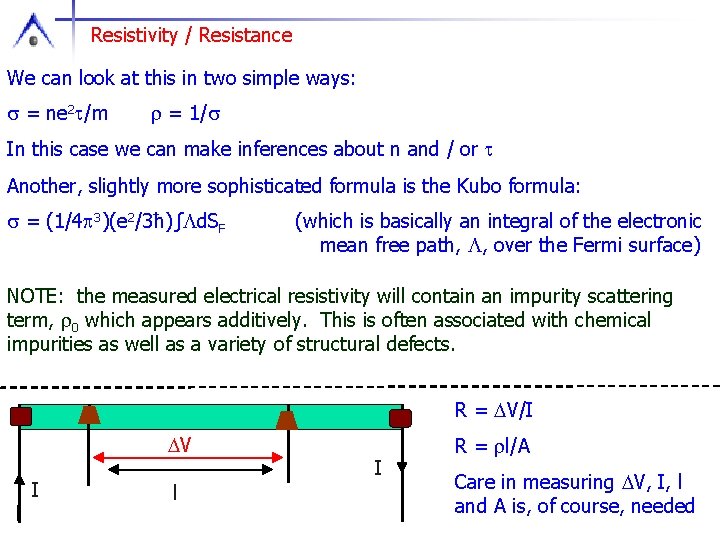
Resistivity / Resistance We can look at this in two simple ways: s = ne 2 t/m r = 1/s In this case we can make inferences about n and / or t Another, slightly more sophisticated formula is the Kubo formula: s = (1/4 p 3)(e 2/3ħ)∫Ld. SF (which is basically an integral of the electronic mean free path, L, over the Fermi surface) NOTE: the measured electrical resistivity will contain an impurity scattering term, r 0 which appears additively. This is often associated with chemical impurities as well as a variety of structural defects. R = DV/I DV I l I R = rl/A Care in measuring DV, I, l and A is, of course, needed

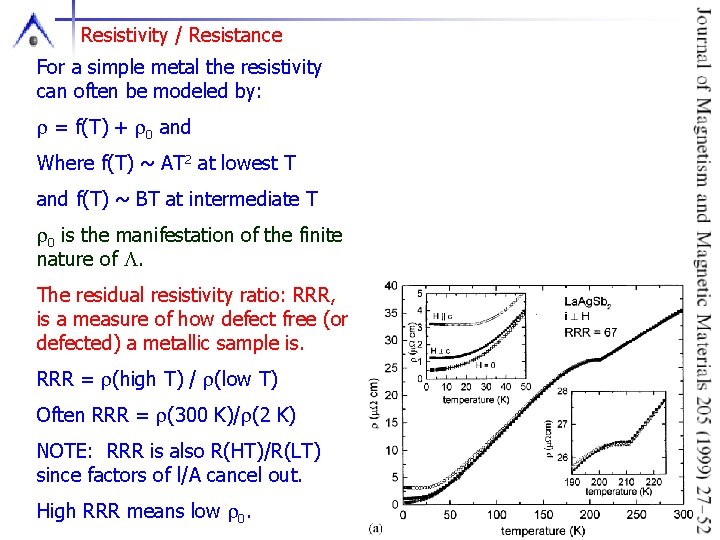
Resistivity / Resistance For a simple metal the resistivity can often be modeled by: r = f(T) + r 0 and Where f(T) ~ AT 2 at lowest T and f(T) ~ BT at intermediate T r 0 is the manifestation of the finite nature of L. The residual resistivity ratio: RRR, is a measure of how defect free (or defected) a metallic sample is. RRR = r(high T) / r(low T) Often RRR = r(300 K)/r(2 K) NOTE: RRR is also R(HT)/R(LT) since factors of l/A cancel out. High RRR means low r 0.

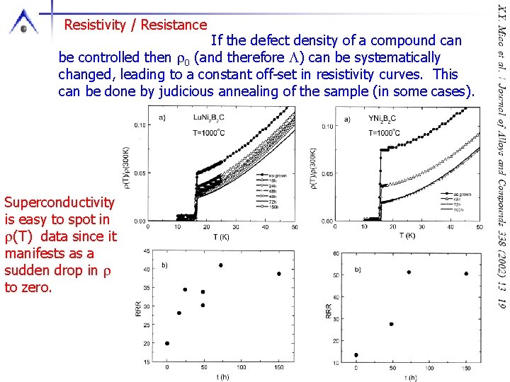
Resistivity / Resistance If the defect density of a compound can be controlled then r 0 (and therefore L) can be systematically changed, leading to a constant off-set in resistivity curves. This can be done by judicious annealing of the sample (in some cases). Superconductivity is easy to spot in r(T) data since it manifests as a sudden drop in r to zero.

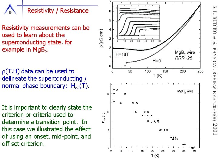
Resistivity / Resistance Resistivity measurements can be used to learn about the superconducting state, for example in Mg. B 2. r(T, H) data can be used to delineate the superconducting / normal phase boundary: Hc 2(T). It is important to clearly state the criterion or criteria used to determine a transition point. In this case we illustrated the effect of using an onset, mid-point, and off-set criterion.

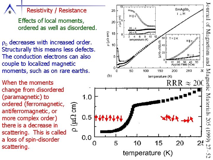
Resistivity / Resistance Effects of local moments, ordered as well as disordered. r 0 decreases with increased order. Structurally this means less defects. The conduction electrons can also couple to localized magnetic moments, such as on rare earths. When the moments change from disordered (paramagnetic) to ordered (ferromagnetic, antiferromagnetic, or more complex order) there is a decrease in scattering. This is called a loss of spin-disorder scattering.

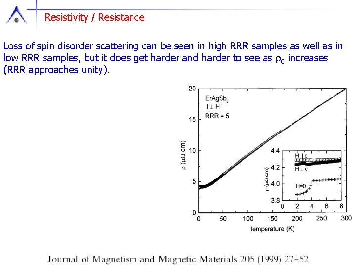
Resistivity / Resistance Loss of spin disorder scattering can be seen in high RRR samples as well as in low RRR samples, but it does get harder and harder to see as r 0 increases (RRR approaches unity).

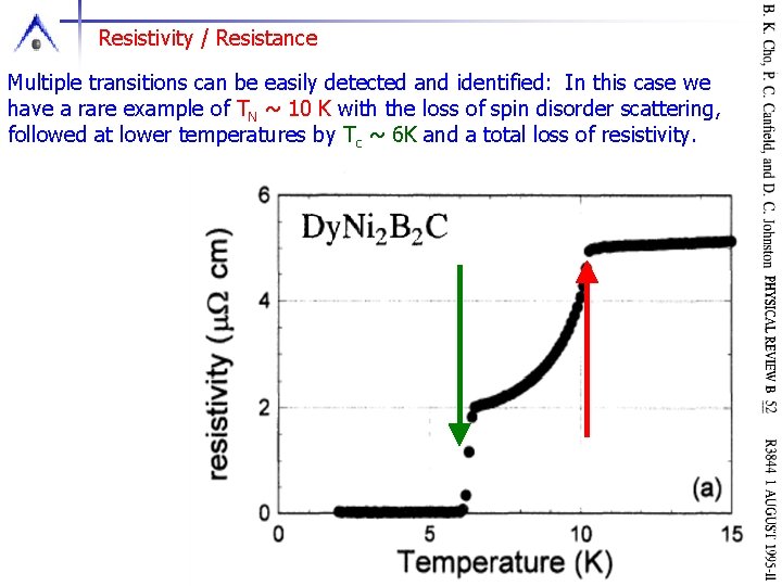
Resistivity / Resistance Multiple transitions can be easily detected and identified: In this case we have a rare example of TN ~ 10 K with the loss of spin disorder scattering, followed at lower temperatures by Tc ~ 6 K and a total loss of resistivity.

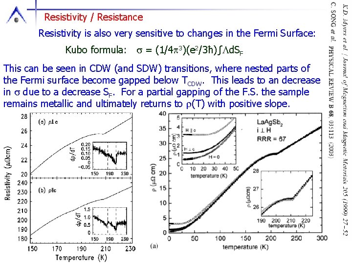
Resistivity / Resistance Resistivity is also very sensitive to changes in the Fermi Surface: Kubo formula: s = (1/4 p 3)(e 2/3ħ)∫Ld. SF This can be seen in CDW (and SDW) transitions, where nested parts of the Fermi surface become gapped below TCDW. This leads to an decrease in s due to a decrease SF. For a partial gapping of the F. S. the sample remains metallic and ultimately returns to r(T) with positive slope.

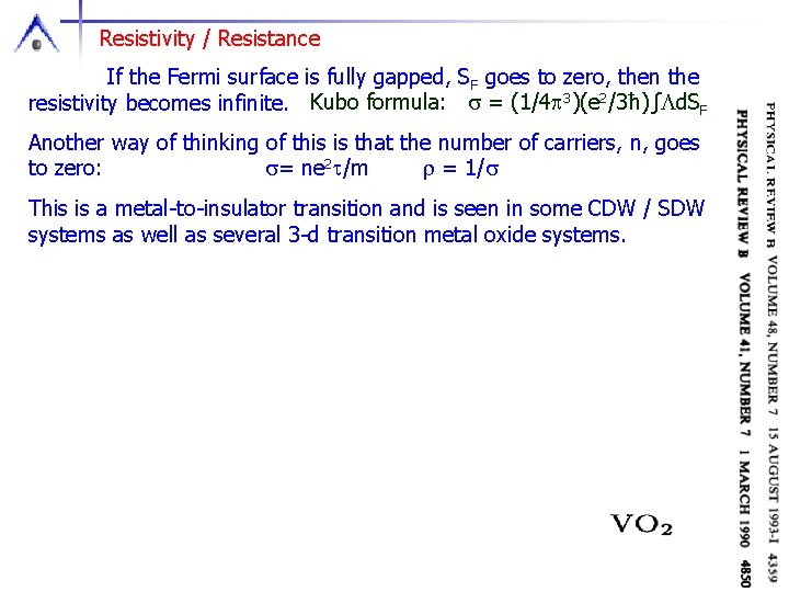
Resistivity / Resistance If the Fermi surface is fully gapped, SF goes to zero, then the resistivity becomes infinite. Kubo formula: s = (1/4 p 3)(e 2/3ħ)∫Ld. SF Another way of thinking of this is that the number of carriers, n, goes to zero: s= ne 2 t/m r = 1/s This is a metal-to-insulator transition and is seen in some CDW / SDW systems as well as several 3 -d transition metal oxide systems.

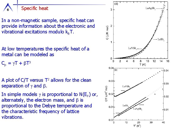
Specific heat In a non-magnetic sample, specific heat can provide information about the electronic and vibrational excitations modulo k. BT. At low temperatures the specific heat of a metal can be modeled as Cp = g. T + b. T 3 A plot of C/T versus T 2 allows for the clean separation of g and b. In simple models g is proportional to N(EF) or, alternately, the electron mass, and b is proportional to the Debye temperature and the characteristic frequency of lattice vibrations.

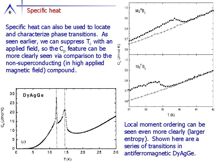
Specific heat can also be used to locate and characterize phase transitions. As seen earlier, we can suppress Tc with an applied field, so the Cp feature can be more clearly seen via comparison to the non-superconducting (in high applied magnetic field) compound. Local moment ordering can be seen even more clearly (larger entropy). Shown here a series of transitions in antiferromagnetic Dy. Ag. Ge.

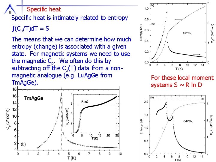
Specific heat is intimately related to entropy ∫(Cp/T)d. T = S The means that we can determine how much entropy (change) is associated with a given state. For magnetic systems we need to use the magnetic Cp. We often do this by subtracting off the Cp(T) data from a nonmagnetic analogue (e. g. Lu. Ag. Ge from Tm. Ag. Ge). For these local moment systems S ~ R ln D

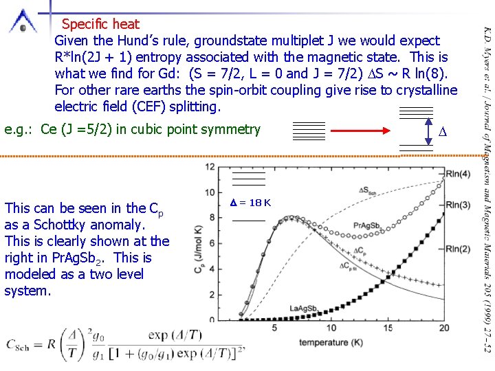
Specific heat Given the Hund’s rule, groundstate multiplet J we would expect R*ln(2 J + 1) entropy associated with the magnetic state. This is what we find for Gd: (S = 7/2, L = 0 and J = 7/2) DS ~ R ln(8). For other rare earths the spin-orbit coupling give rise to crystalline electric field (CEF) splitting. e. g. : Ce (J =5/2) in cubic point symmetry This can be seen in the Cp as a Schottky anomaly. This is clearly shown at the right in Pr. Ag. Sb 2. This is modeled as a two level system. D = 18 K D

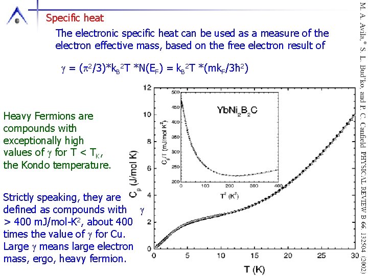
Specific heat The electronic specific heat can be used as a measure of the electron effective mass, based on the free electron result of g = (p 2/3)*k. B 2 T *N(EF) = k. B 2 T *(mk. F/3ħ 2) Heavy Fermions are compounds with exceptionally high values of g for T < TK, the Kondo temperature. Strictly speaking, they are defined as compounds with g > 400 m. J/mol-K 2, about 400 times the value of g for Cu. Large g means large electron mass, ergo, heavy fermion.

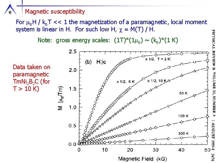
Magnetic susceptibility For m. BH / k. BT << 1 the magnetization of a paramagnetic, local moment system is linear in H. For such low H, c = M(T) / H. Note: gross energy scales: (1 T)*(1 m. B) ~ (k. B)*(1 K) Data taken on paramagnetic Tm. Ni 2 B 2 C (for T > 10 K)

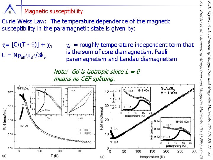
Magnetic susceptibility Curie Weiss Law: The temperature dependence of the magnetic susceptibility in the paramagnetic state is given by: c= [C/(T - q)] + c 0 C = Npeff 2 m. B 2/3 k. B c 0 = roughly temperature independent term that is the sum of core diamagnetism, Pauli paramagnetism and Landau diamagnetism Note: Gd is isotropic since L = 0 means no CEF splitting.

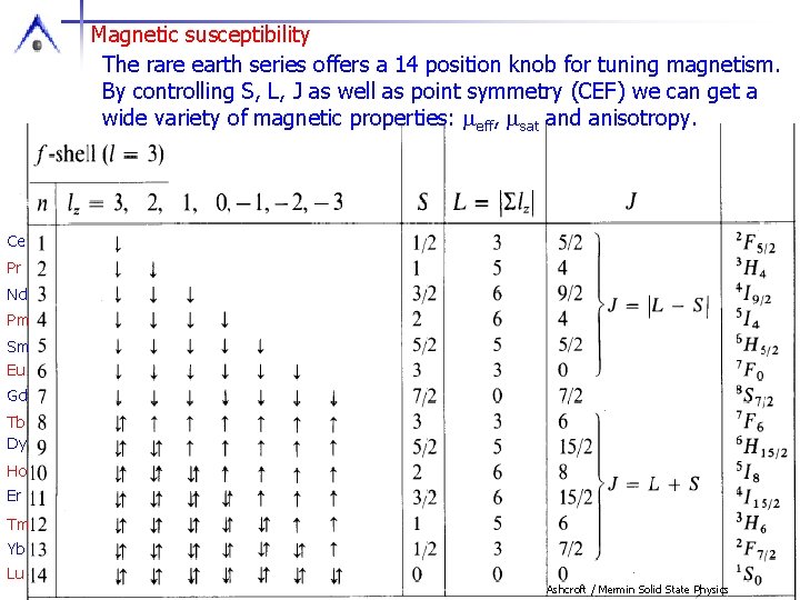
Magnetic susceptibility The rare earth series offers a 14 position knob for tuning magnetism. By controlling S, L, J as well as point symmetry (CEF) we can get a wide variety of magnetic properties: meff, msat and anisotropy. Ce Pr Nd Pm Sm Eu Gd Tb Dy Ho Er Tm Yb Lu Ashcroft / Mermin Solid State Physics

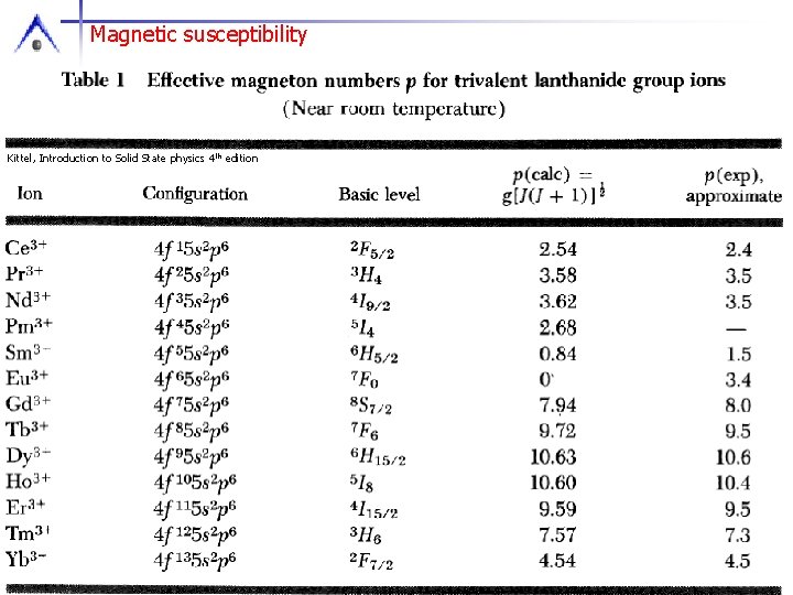
Magnetic susceptibility Kittel, Introduction to Solid State physics 4 th edition

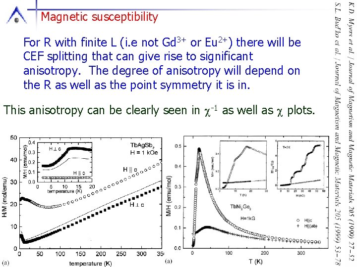
Magnetic susceptibility For R with finite L (i. e not Gd 3+ or Eu 2+) there will be CEF splitting that can give rise to significant anisotropy. The degree of anisotropy will depend on the R as well as the point symmetry it is in. This anisotropy can be clearly seen in c-1 as well as c plots.

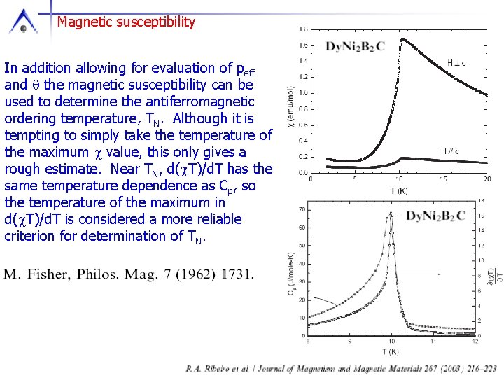
Magnetic susceptibility In addition allowing for evaluation of peff and q the magnetic susceptibility can be used to determine the antiferromagnetic ordering temperature, TN. Although it is tempting to simply take the temperature of the maximum c value, this only gives a rough estimate. Near TN, d(c. T)/d. T has the same temperature dependence as Cp, so the temperature of the maximum in d(c. T)/d. T is considered a more reliable criterion for determination of TN.

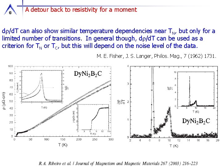
A detour back to resistivity for a moment dr/d. T can also show similar temperature dependencies near TN, but only for a limited number of transitions. In general though, dr/d. T can be used as a criterion for TN or TC, but this will depend on the noise level of the data. M. E. Fisher, J. S. Langer, Philos. Mag. , 7 (1962) 1731.

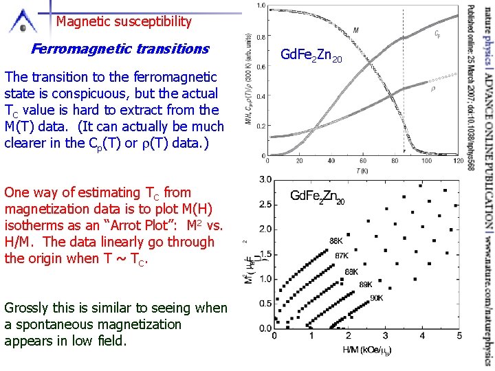
Magnetic susceptibility Ferromagnetic transitions The transition to the ferromagnetic state is conspicuous, but the actual TC value is hard to extract from the M(T) data. (It can actually be much clearer in the Cp(T) or r(T) data. ) One way of estimating TC from magnetization data is to plot M(H) isotherms as an “Arrot Plot”: M 2 vs. H/M. The data linearly go through the origin when T ~ TC. Grossly this is similar to seeing when a spontaneous magnetization appears in low field. Gd. Fe 2 Zn 20

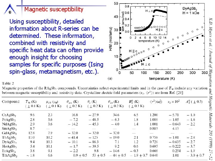
Magnetic susceptibility Using susceptibility, detailed information about R-series can be determined. These information, combined with resistivity and specific heat data can often provide enough insight for choosing samples for specific purposes (Ising spin-glass, metamagnetism, etc. ).

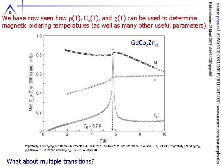
We have now seen how r(T), Cp(T), and c(T) can be used to determine magnetic ordering temperatures (as well as many other useful parameters). Gd. Co 2 Zn 20 What about multiple transitions?

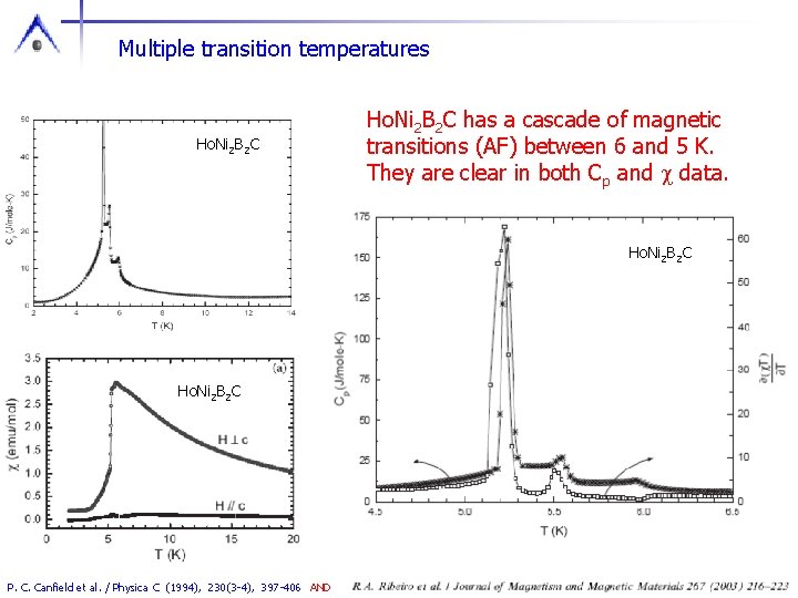
Multiple transition temperatures Ho. Ni 2 B 2 C has a cascade of magnetic transitions (AF) between 6 and 5 K. They are clear in both Cp and c data. Ho. Ni 2 B 2 C P. C. Canfield et al. / Physica C (1994), 230(3 -4), 397 -406 AND

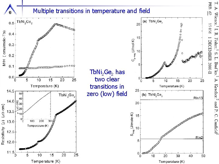
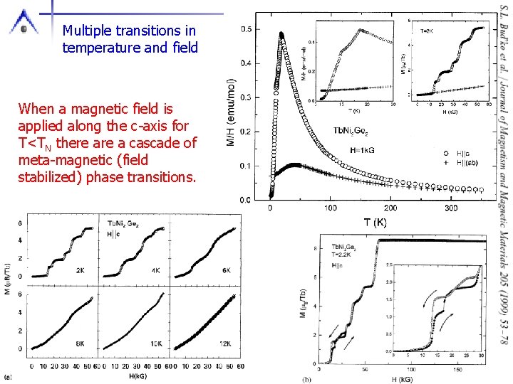
Multiple transitions in temperature and field Tb. Ni 2 Ge 2 has two clear transitions in zero (low) field

Multiple transitions in temperature and field When a magnetic field is applied along the c-axis for T<TN there a cascade of meta-magnetic (field stabilized) phase transitions.

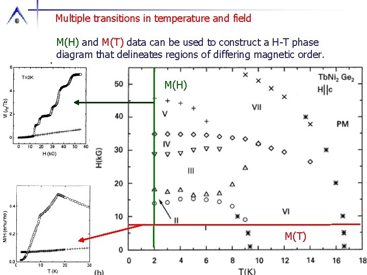
Multiple transitions in temperature and field M(H) and M(T) data can be used to construct a H-T phase diagram that delineates regions of differing magnetic order. M(H) M(T)

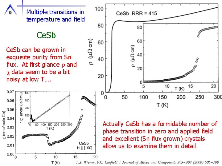
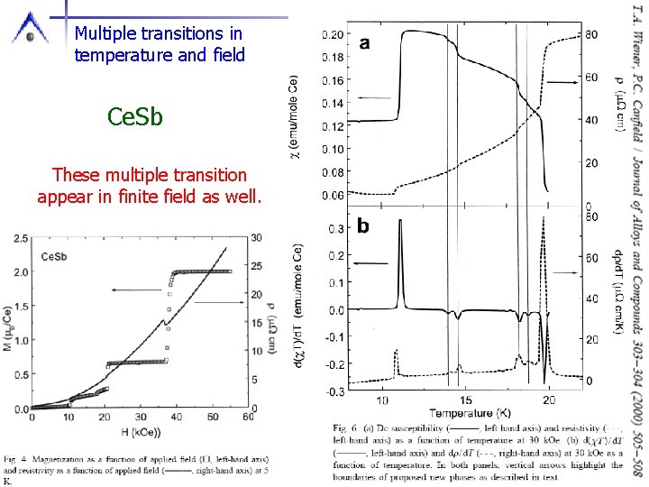
Multiple transitions in temperature and field Ce. Sb can be grown in exquisite purity from Sn flux. At first glance r and c data seem to be a bit noisy at low T…. Actually Ce. Sb has a formidable number of phase transition in zero and applied field and excellent (Sn flux grown) crystals allow us to examine them in detail.

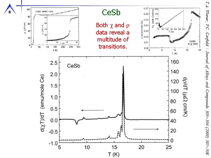
Ce. Sb Both c and r data reveal a multitude of transitions.

Multiple transitions in temperature and field Ce. Sb These multiple transition appear in finite field as well.

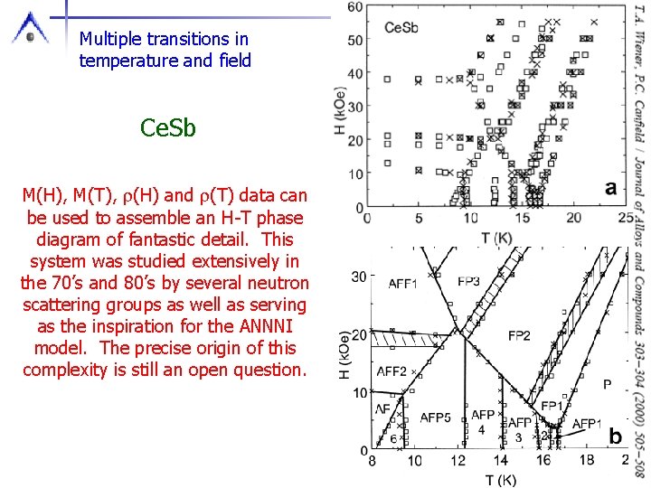
Multiple transitions in temperature and field Ce. Sb M(H), M(T), r(H) and r(T) data can be used to assemble an H-T phase diagram of fantastic detail. This system was studied extensively in the 70’s and 80’s by several neutron scattering groups as well as serving as the inspiration for the ANNNI model. The precise origin of this complexity is still an open question.

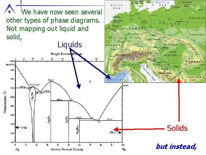
We have now seen several other types of phase diagrams. Not mapping out liquid and solid, Liquids Solids but instead,

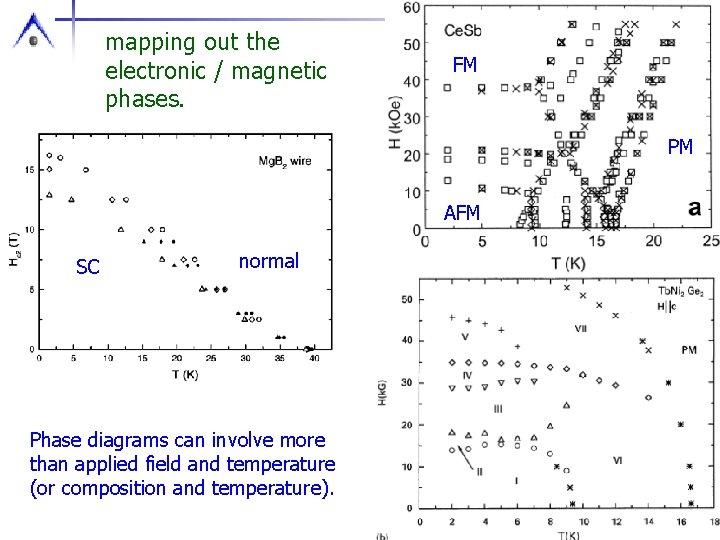
mapping out the electronic / magnetic phases. FM PM AFM SC normal Phase diagrams can involve more than applied field and temperature (or composition and temperature).

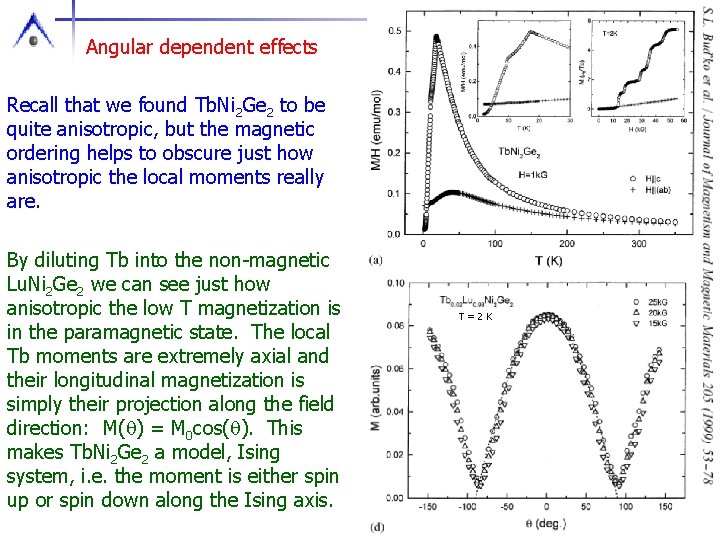
Angular dependent effects Recall that we found Tb. Ni 2 Ge 2 to be quite anisotropic, but the magnetic ordering helps to obscure just how anisotropic the local moments really are. By diluting Tb into the non-magnetic Lu. Ni 2 Ge 2 we can see just how anisotropic the low T magnetization is in the paramagnetic state. The local Tb moments are extremely axial and their longitudinal magnetization is simply their projection along the field direction: M(q) = M 0 cos(q). This makes Tb. Ni 2 Ge 2 a model, Ising system, i. e. the moment is either spin up or spin down along the Ising axis. T=2 K

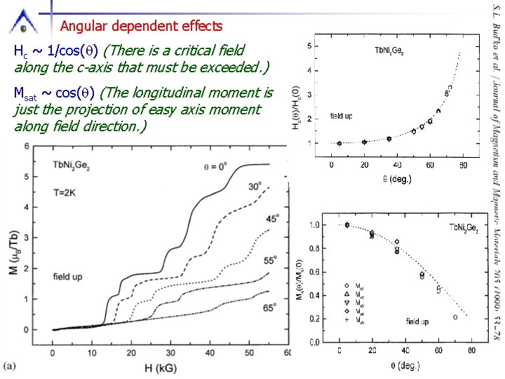
Angular dependent effects Hc ~ 1/cos(q) (There is a critical field along the c-axis that must be exceeded. ) Msat ~ cos(q) (The longitudinal moment is just the projection of easy axis moment along field direction. )

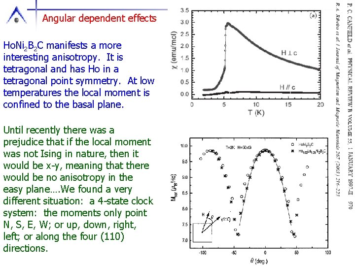
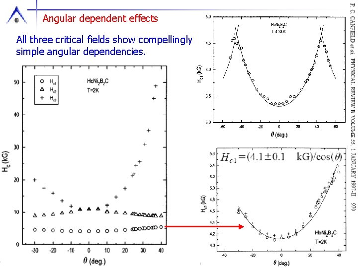
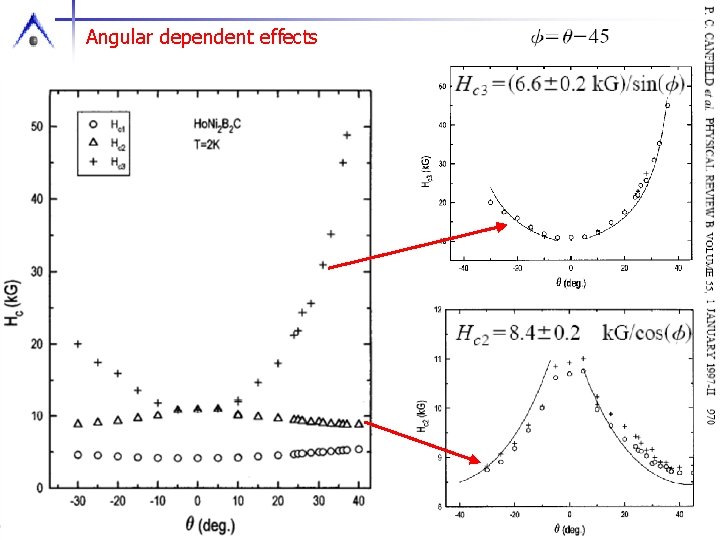
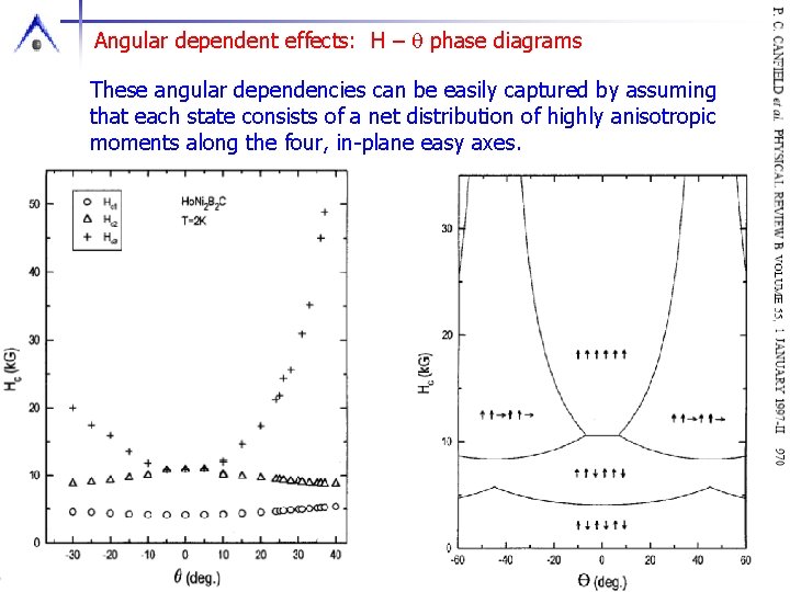
Angular dependent effects Ho. Ni 2 B 2 C manifests a more interesting anisotropy. It is tetragonal and has Ho in a tetragonal point symmetry. At low temperatures the local moment is confined to the basal plane. Until recently there was a prejudice that if the local moment was not Ising in nature, then it would be x-y, meaning that there would be no anisotropy in the easy plane…. We found a very different situation: a 4 -state clock system: the moments only point N, S, E, W; or up, down, right, left; or along the four (110) directions.

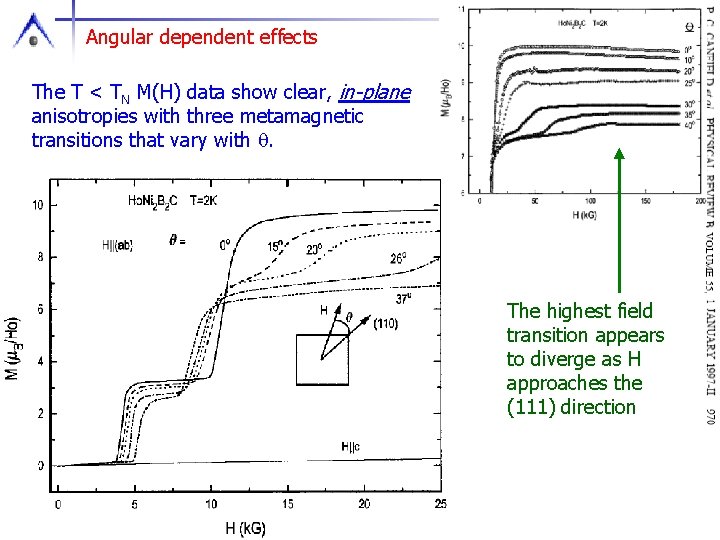
Angular dependent effects The T < TN M(H) data show clear, in-plane anisotropies with three metamagnetic transitions that vary with q. The highest field transition appears to diverge as H approaches the (111) direction

Angular dependent effects All three critical fields show compellingly simple angular dependencies.

Angular dependent effects

Angular dependent effects: H – q phase diagrams These angular dependencies can be easily captured by assuming that each state consists of a net distribution of highly anisotropic moments along the four, in-plane easy axes.

Summary This lecture has reviewed how to map, identify and start to describe regions of H-T (and in the end H-q) phase space with three simple measurement techniques: r(T, H, q), Cp(T, H, q), M(T, H, q). These techniques combined with the ability to design, discovery, and grow novel compounds opens the way to the discovery and description of novel physics.

What else can we do? (part 1) More advanced data with basically the same measurements: Magneto-transport r(H) and Kohler’s rule Hall efffect Quantum oscillations d. Hv. A measurements in M(H) Sd. H measurements in r(H) Other measurements that are basic and useful: Thermoelectric power Thermal Conductivity

What else can we do? (part 2) Extremes that help us learn more by changing energy ratios: Low T: down to 1. 5 K, down to 0. 3 K , down to 0. 03 K. Each gets harder and more expensive. High d. c. magnetic field: 5 T, 10 T, 15 T, 20 T. Each step doubles cost (or more) Pulsed magnetic fields: 30 T, 60 T, 90 T Extremes help us learn more by controllably perturbing the sample: Pressure: use of hydrostatic pressure to tune compounds is clean and useful. 10 – 30 kbar is not too hard, 30 – 100 kbar is difficult, and greater than 100 kbar is very difficult. Resistivity under pressure is the easiest measurement. Low pressure (~ 10 kbar) magnetic susceptibility, c, is not too hard either. Some of these measurements can be done in your own lab, some with friends, some at specialized facilities.

That’s All Folks