Endogeneity in PLSSEM The Gaussian Copula Approach http

Endogeneity in PLS-SEM: The Gaussian Copula Approach http: //journals. ama. org/doi/10. 1509/jim. 17. 0151 Hult, G. T. M. , Hair, J. F. , Proksch, D. , Sarstedt, M. , Pinkwart, A. , and Ringle, C. M. (2018). Addressing Endogeneity in International Marketing Applications of Partial Least Squares Structural Equation Modeling, Journal of International Marketing, forthcoming.

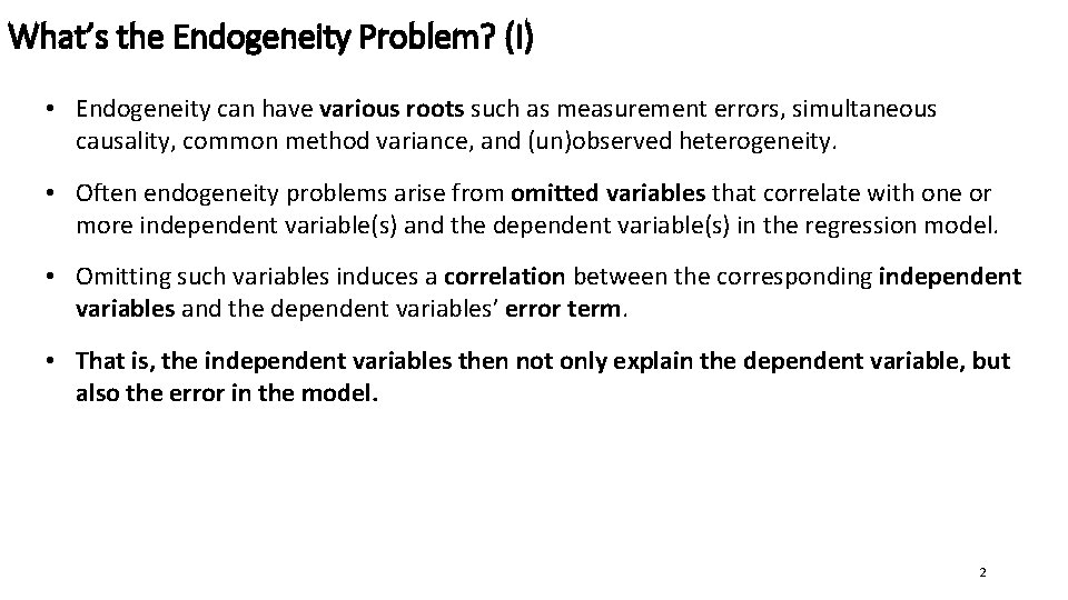
What’s the Endogeneity Problem? (I) • Endogeneity can have various roots such as measurement errors, simultaneous causality, common method variance, and (un)observed heterogeneity. • Often endogeneity problems arise from omitted variables that correlate with one or more independent variable(s) and the dependent variable(s) in the regression model. • Omitting such variables induces a correlation between the corresponding independent variables and the dependent variables’ error term. • That is, the independent variables then not only explain the dependent variable, but also the error in the model. 2

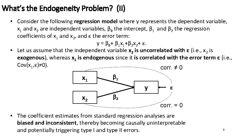
What’s the Endogeneity Problem? (II) • Consider the following regression model where y represents the dependent variable, x 1 and x 2 are independent variables, β 0 the intercept, β 1 and β 2 the regression coefficients of x 1 and x 2, and ε the error term: y = β 0+ β 1 x 1+β 2 x 2+ ε. • Let us assume that the independent variable x 2 is uncorrelated with ε (i. e. , x 2 is exogenous), whereas x 1 is endogenous since it is correlated with the error term ε (i. e. , Cov(x 1, ε)≠ 0). corr. ≠ 0 x 1 1 y x 2 ε 2 corr. = 0 • The coefficient estimates from standard regression analyses are biased and inconsistent, thereby becoming causally uninterpretable and potentially triggering type I and type II errors. 3

On the Relevance Assessment in PLS-SEM • Dealing with endogeneity has been extensively discussed in the literature, especially with respect to different forms of regression and panel models, as well as conjoint analysis. • While several studies have discussed endogeneity in the context of factor-based SEM, there is a paucity of research on this topic in PLS-SEM. • Some researchers even claim that PLS-SEM does not allow for addressing endogeneity at all. This assertion is astonishing and inaccurate given that PLS-SEM is grounded in regression analysis, for which numerous approaches for handling endogeneity exist. • Hence, research must address when and how to address endogeneity in PLS-SEM. 4

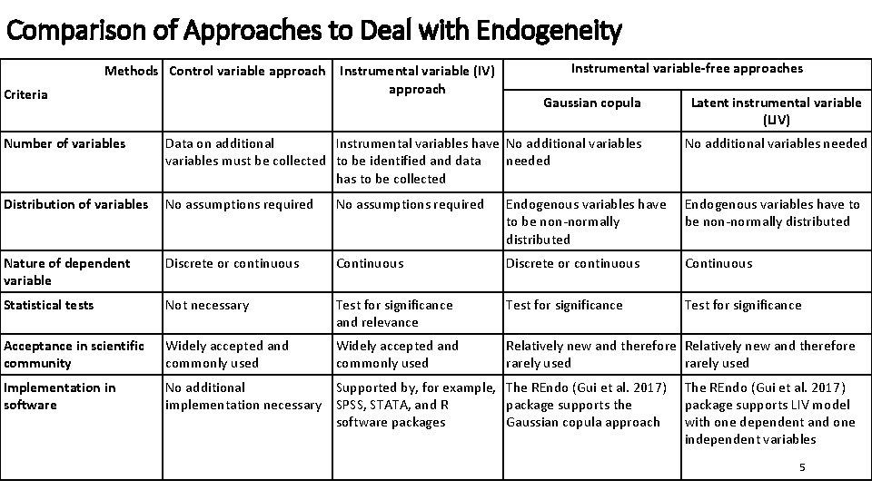
Comparison of Approaches to Deal with Endogeneity Methods Control variable approach Criteria Instrumental variable (IV) approach Instrumental variable-free approaches Gaussian copula Latent instrumental variable (LIV) Number of variables Data on additional Instrumental variables have No additional variables must be collected to be identified and data needed has to be collected No additional variables needed Distribution of variables No assumptions required Endogenous variables have to be non-normally distributed Nature of dependent variable Discrete or continuous Continuous Statistical tests Not necessary Test for significance and relevance Test for significance Acceptance in scientific community Widely accepted and commonly used Relatively new and therefore rarely used Implementation in software No additional Supported by, for example, The REndo (Gui et al. 2017) implementation necessary SPSS, STATA, and R package supports the software packages Gaussian copula approach The REndo (Gui et al. 2017) package supports LIV model with one dependent and one independent variables 5

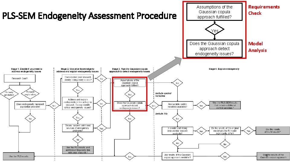
PLS-SEM Endogeneity Assessment Procedure Assumptions of the Gaussian copula approach fulfilled? Requirements Check Yes Does the Gaussian copula approach detect endogeneity issues? Model Analysis 6

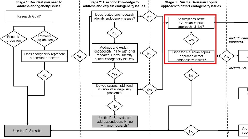
7

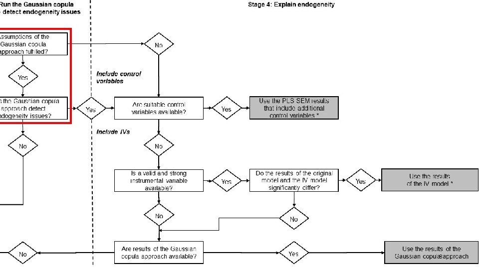
8

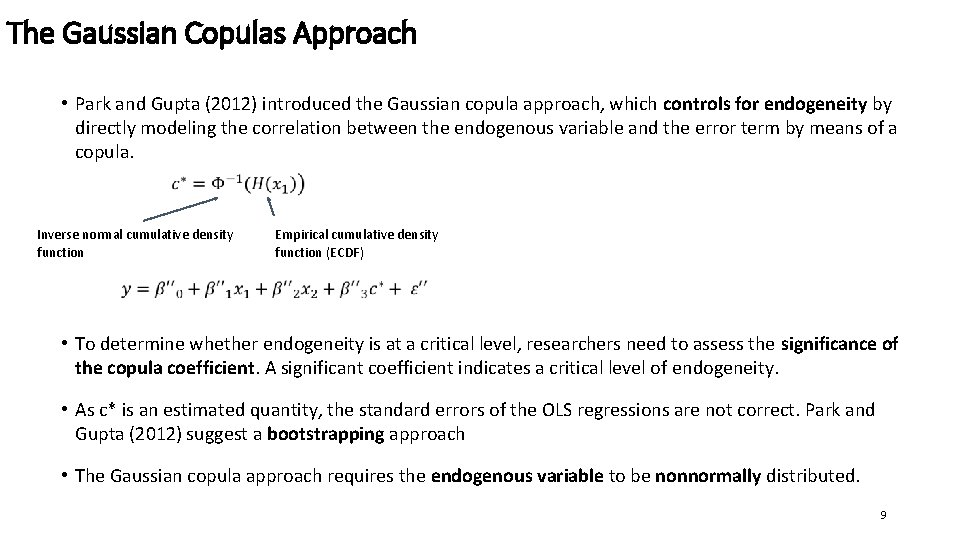
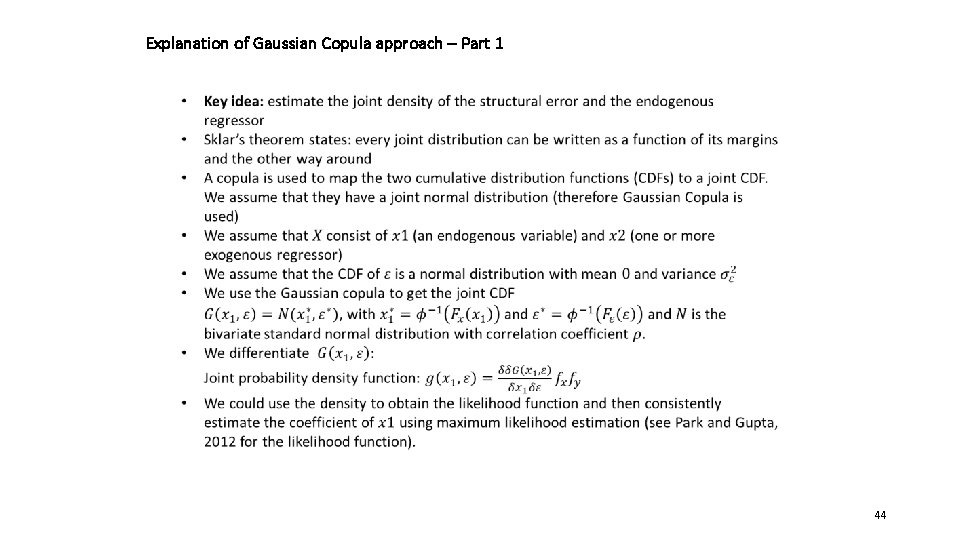
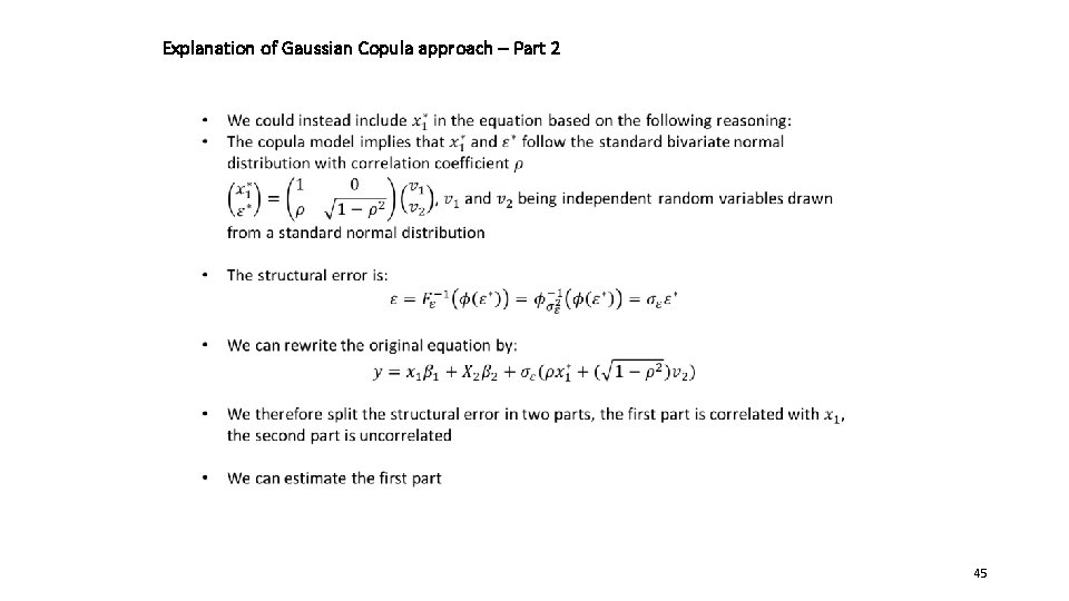
The Gaussian Copulas Approach • Park and Gupta (2012) introduced the Gaussian copula approach, which controls for endogeneity by directly modeling the correlation between the endogenous variable and the error term by means of a copula. Inverse normal cumulative density function Empirical cumulative density function (ECDF) • To determine whether endogeneity is at a critical level, researchers need to assess the significance of the copula coefficient. A significant coefficient indicates a critical level of endogeneity. • As c* is an estimated quantity, the standard errors of the OLS regressions are not correct. Park and Gupta (2012) suggest a bootstrapping approach • The Gaussian copula approach requires the endogenous variable to be nonnormally distributed. 9

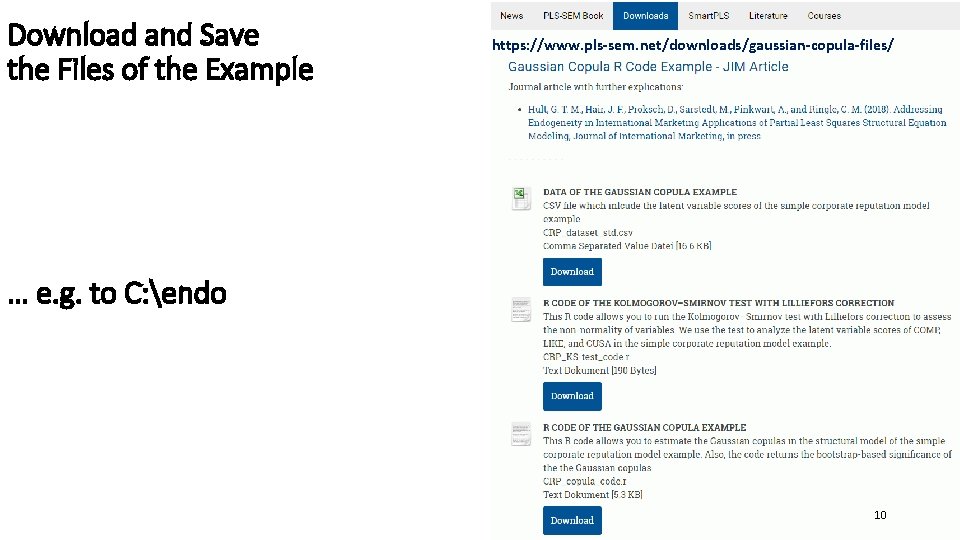
Download and Save the Files of the Example https: //www. pls-sem. net/downloads/gaussian-copula-files/ … e. g. to C: endo 10

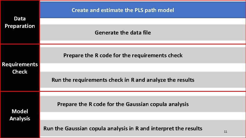
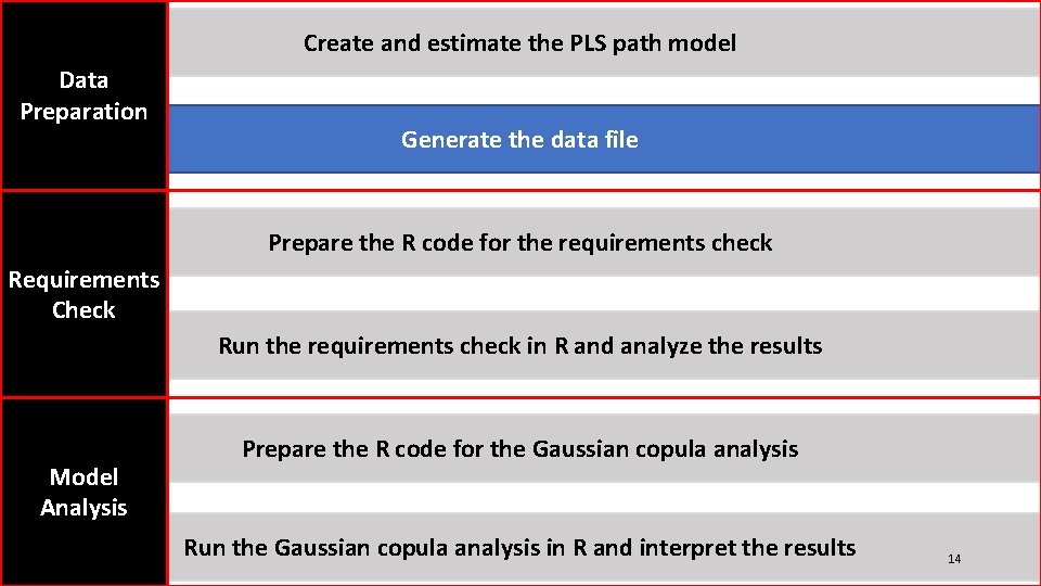
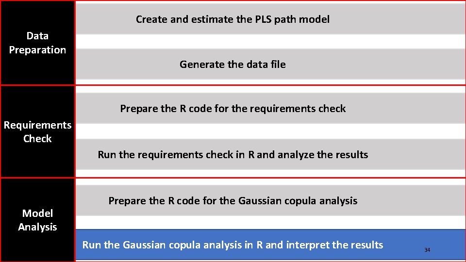
Create and estimate the PLS path model Data Preparation Generate the data file Prepare the R code for the requirements check Requirements Check Run the requirements check in R and analyze the results Model Analysis Prepare the R code for the Gaussian copula analysis Run the Gaussian copula analysis in R and interpret the results 11

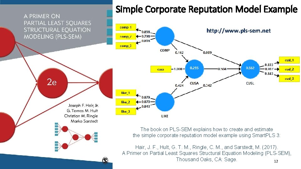
Simple Corporate Reputation Model Example http: //www. pls-sem. net The book on PLS-SEM explains how to create and estimate the simple corporate reputation model example using Smart. PLS 3: Hair, J. F. , Hult, G. T. M. , Ringle, C. M. , and Sarstedt, M. (2017). A Primer on Partial Least Squares Structural Equation Modeling (PLS-SEM), Thousand Oaks, CA: Sage. 12

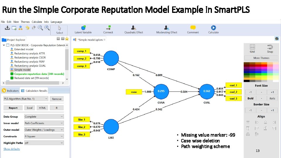
Run the Simple Corporate Reputation Model Example in Smart. PLS • Missing value marker: -99 • Case wise deletion • Path weighting scheme 13

Create and estimate the PLS path model Data Preparation Generate the data file Prepare the R code for the requirements check Requirements Check Run the requirements check in R and analyze the results Model Analysis Prepare the R code for the Gaussian copula analysis Run the Gaussian copula analysis in R and interpret the results 14

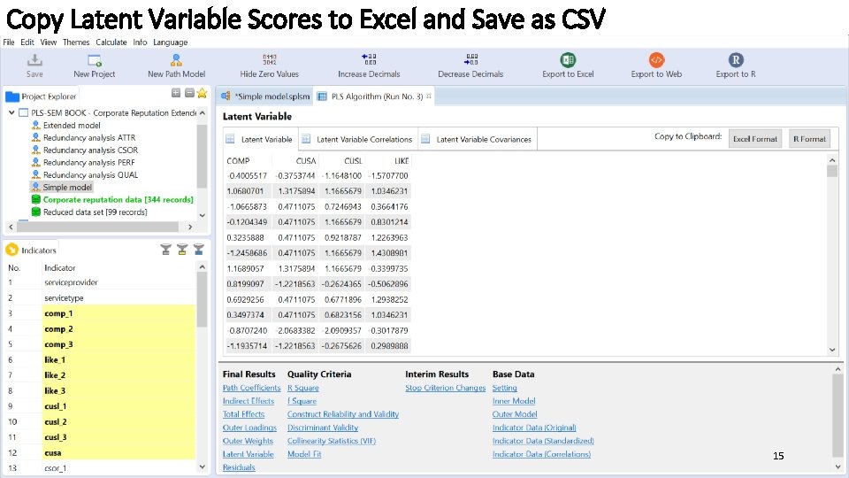
Copy Latent Variable Scores to Excel and Save as CSV 15

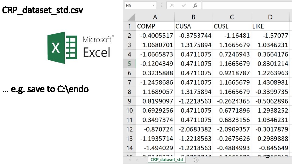
CRP_dataset_std. csv … e. g. save to C: endo 16

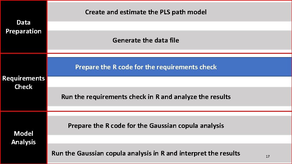
Create and estimate the PLS path model Data Preparation Generate the data file Prepare the R code for the requirements check Requirements Check Run the requirements check in R and analyze the results Model Analysis Prepare the R code for the Gaussian copula analysis Run the Gaussian copula analysis in R and interpret the results 17

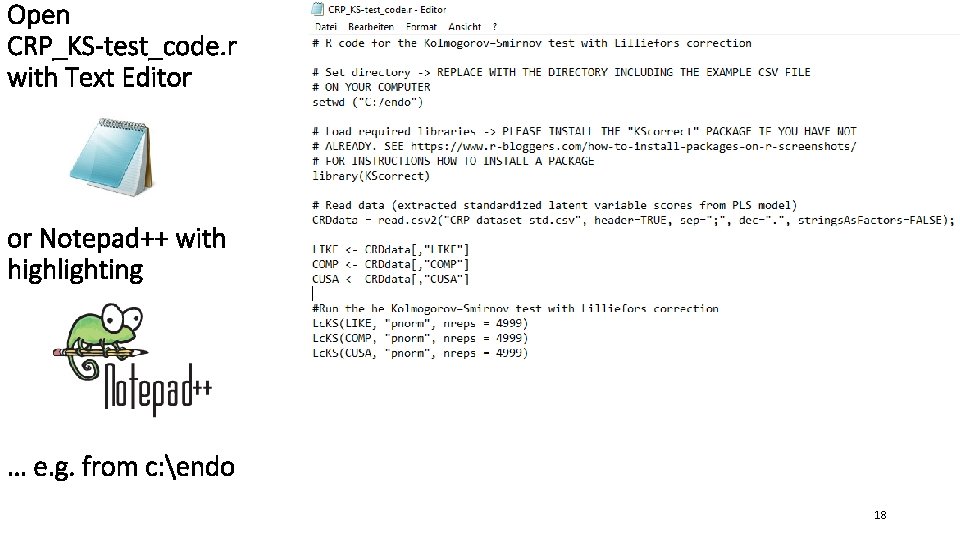
Open CRP_KS-test_code. r with Text Editor or Notepad++ with highlighting … e. g. from c: endo 18

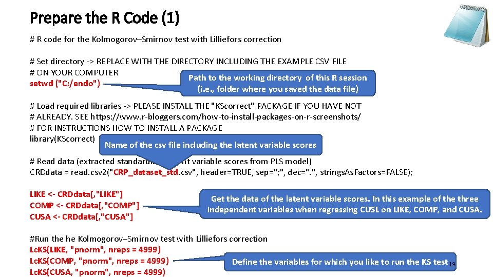
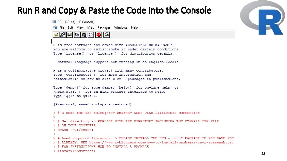
Prepare the R Code (1) # R code for the Kolmogorov–Smirnov test with Lilliefors correction # Set directory -> REPLACE WITH THE DIRECTORY INCLUDING THE EXAMPLE CSV FILE # ON YOUR COMPUTER Path to the working directory of this R session setwd ("C: /endo") (i. e. , folder where you saved the data file) # Load required libraries -> PLEASE INSTALL THE "KScorrect" PACKAGE IF YOU HAVE NOT # ALREADY. SEE https: //www. r-bloggers. com/how-to-install-packages-on-r-screenshots/ # FOR INSTRUCTIONS HOW TO INSTALL A PACKAGE library(KScorrect) Name of the csv file including the latent variable scores # Read data (extracted standardized latent variable scores from PLS model) CRDdata = read. csv 2("CRP_dataset_std. csv", header=TRUE, sep="; ", dec=". ", strings. As. Factors=FALSE); LIKE <- CRDdata[, "LIKE"] COMP <- CRDdata[, "COMP"] CUSA <- CRDdata[, "CUSA"] Get the data of the latent variable scores. In this example of the three independent variables when regressing CUSL on LIKE, COMP, and CUSA. #Run the he Kolmogorov–Smirnov test with Lilliefors correction Lc. KS(LIKE, "pnorm", nreps = 4999) Lc. KS(COMP, "pnorm", nreps = 4999) Define the variables for which you like to run the KS test 19 Lc. KS(CUSA, "pnorm", nreps = 4999)

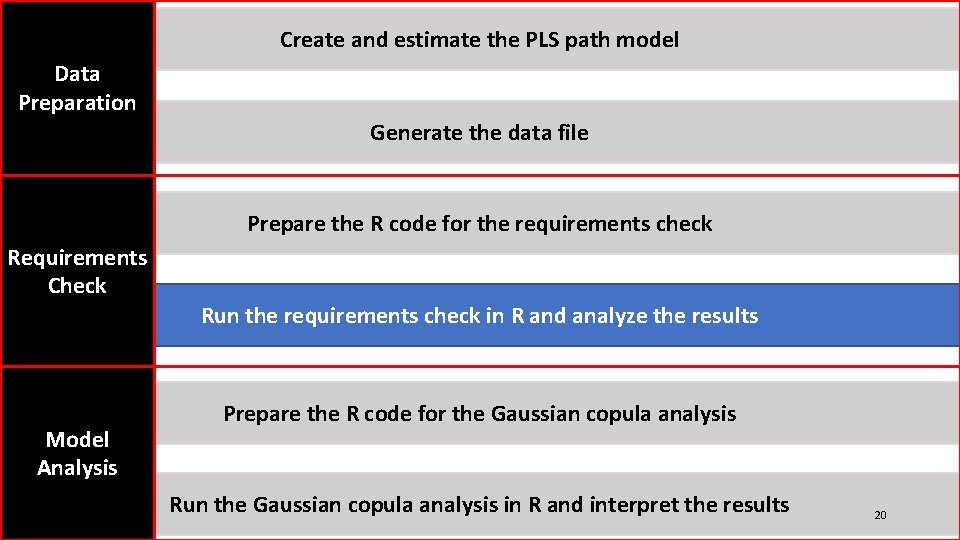
Create and estimate the PLS path model Data Preparation Generate the data file Prepare the R code for the requirements check Requirements Check Run the requirements check in R and analyze the results Model Analysis Prepare the R code for the Gaussian copula analysis Run the Gaussian copula analysis in R and interpret the results 20

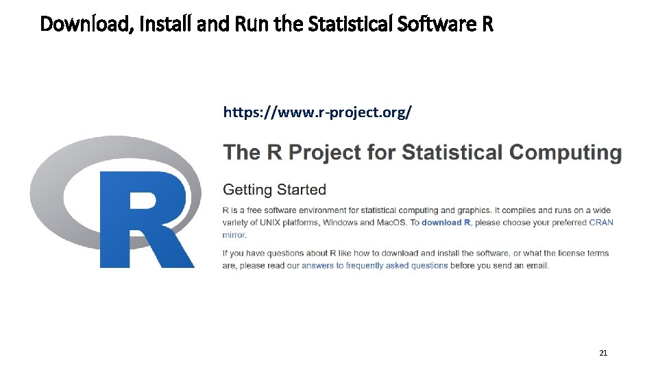
Download, Install and Run the Statistical Software R https: //www. r-project. org/ 21

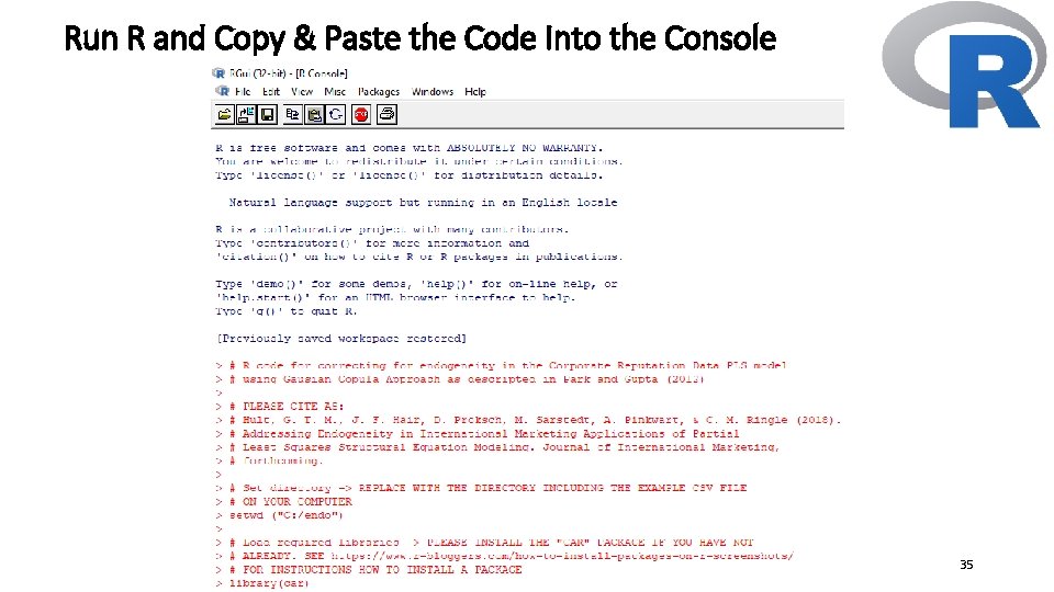
Run R and Copy & Paste the Code Into the Console 22

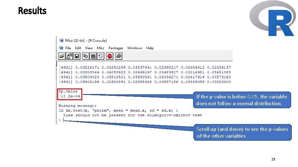
Results If the p-value is below 0. 05, the variable does not follow a normal distribution. Scroll up (and down) to see the p-values of the other variables 23

Requirements Check Before Running Gaussian Copulas • Before initiating the Gaussian copula approach to meet its assumptions, we first verify if the variables, which potentially exhibit endogeneity, are non-normally distributed. • We do so by running the Kolmogorov–Smirnov test with Lilliefors correction (Sarstedt and Mooi 2014) on the standardized composite scores of COMP, LIKE, and CUSA, which the PLS path model estimation provides. • If the p-value is below 0. 05, the variable does not follow a normal distribution. • The results show that none of the constructs has normally distributed scores, which allows us to consider them endogenous in the Gaussian copula analysis. 24

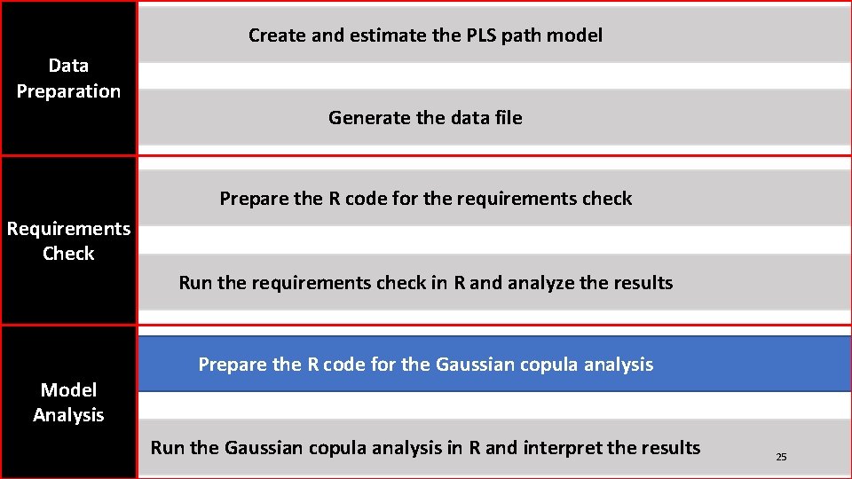
Create and estimate the PLS path model Data Preparation Generate the data file Prepare the R code for the requirements check Requirements Check Run the requirements check in R and analyze the results Model Analysis Prepare the R code for the Gaussian copula analysis Run the Gaussian copula analysis in R and interpret the results 25

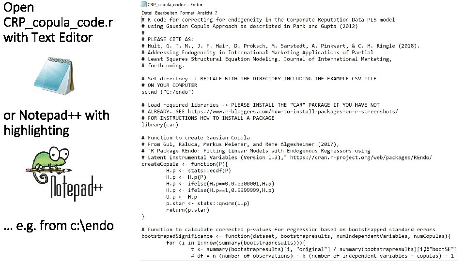
Open CRP_copula_code. r with Text Editor or Notepad++ with highlighting … e. g. from c: endo 26

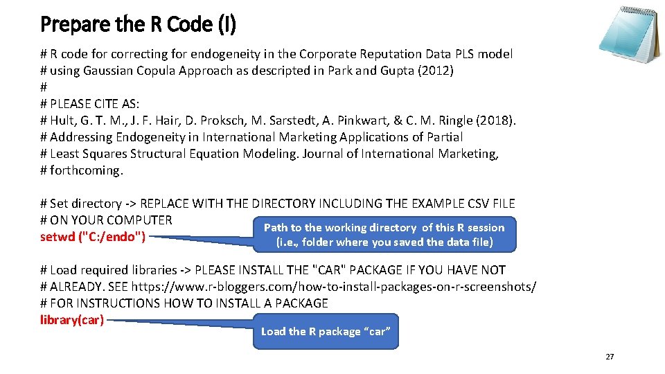
Prepare the R Code (I) # R code for correcting for endogeneity in the Corporate Reputation Data PLS model # using Gaussian Copula Approach as descripted in Park and Gupta (2012) # # PLEASE CITE AS: # Hult, G. T. M. , J. F. Hair, D. Proksch, M. Sarstedt, A. Pinkwart, & C. M. Ringle (2018). # Addressing Endogeneity in International Marketing Applications of Partial # Least Squares Structural Equation Modeling. Journal of International Marketing, # forthcoming. # Set directory -> REPLACE WITH THE DIRECTORY INCLUDING THE EXAMPLE CSV FILE # ON YOUR COMPUTER Path to the working directory of this R session setwd ("C: /endo") (i. e. , folder where you saved the data file) # Load required libraries -> PLEASE INSTALL THE "CAR" PACKAGE IF YOU HAVE NOT # ALREADY. SEE https: //www. r-bloggers. com/how-to-install-packages-on-r-screenshots/ # FOR INSTRUCTIONS HOW TO INSTALL A PACKAGE library(car) Load the R package “car” 27

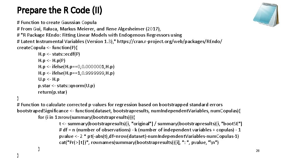
Prepare the R Code (II) # Function to create Gaussian Copula # From Gui, Raluca, Markus Meierer, and Rene Algesheimer (2017), # "R Package REndo: Fitting Linear Models with Endogenous Regressors using # Latent Instrumental Variables (Version 1. 3), " https: //cran. r-project. org/web/packages/REndo/ create. Copula <- function(P){ H. p <- stats: : ecdf(P) H. p <- H. p(P) H. p <- ifelse(H. p==0, 0. 0000001, H. p) H. p <- ifelse(H. p==1, 0. 9999999, H. p) U. p <- H. p p. star <- stats: : qnorm(U. p) return(p. star) } # Function to calculate corrected p-values for regression based on bootstrapped standard errors bootstraped. Significance <- function(dataset, bootstrapresults, num. Independent. Variables, num. Copulas){ for (i in 1: nrow(summary(bootstrapresults))){ t <- summary(bootstrapresults)[i, "original"] / summary(bootstrapresults)[i, "boot. SE"] # df = n (number of observations) - k (number of independent variables + copulas) - 1 pvalue <- 2 * pt(-abs(t), df=nrow(dataset)-num. Independent. Variables-num. Copulas-1) cat("Pr(>|t|)", rownames(summary(bootstrapresults))[i], ": ", pvalue, "n") } } 28

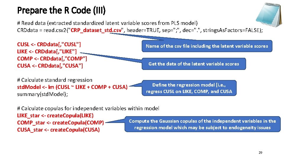
Prepare the R Code (III) # Read data (extracted standardized latent variable scores from PLS model) CRDdata = read. csv 2("CRP_dataset_std. csv", header=TRUE, sep="; ", dec=". ", strings. As. Factors=FALSE); CUSL <- CRDdata[, "CUSL"] LIKE <- CRDdata[, "LIKE"] COMP <- CRDdata[, "COMP"] CUSA <- CRDdata[, "CUSA"] # Calculate standard regression std. Model <- lm (CUSL ~ LIKE + COMP + CUSA) summary(std. Model); Name of the csv file including the latent variable scores Get the data of the latent variable scores Define the regression model (i. e. , regress CUSL on LIKE, COMP, and CUSA # Calculate copulas for independent variables within model LIKE_star <- create. Copula(LIKE) Compute the Gaussian copulas of the independent variables in the COMP_star <- create. Copula(COMP) regression model which may be subject to endogeneity issues CUSA_star <- create. Copula(CUSA) 29

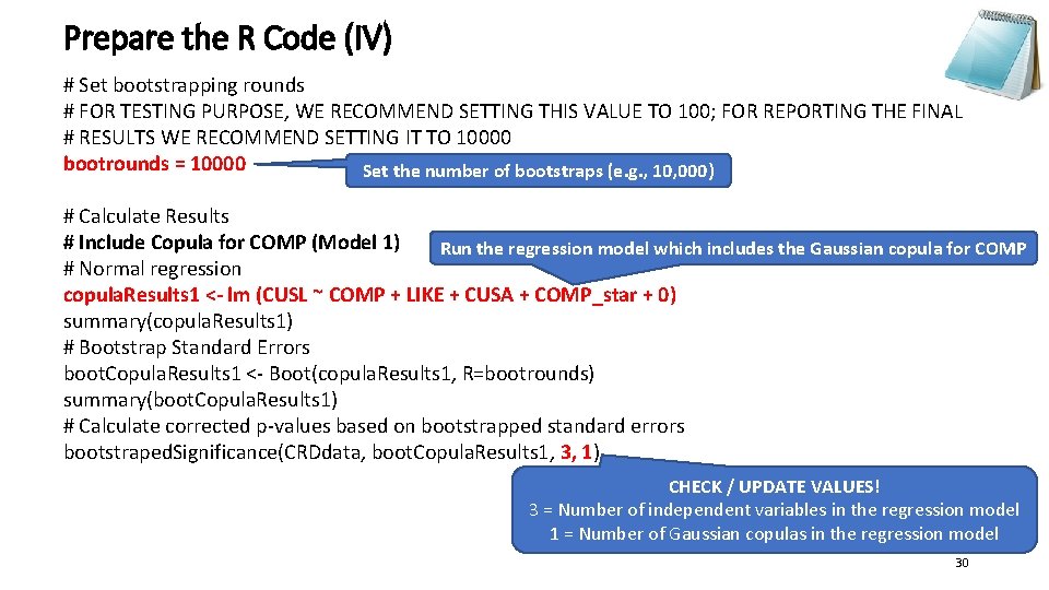
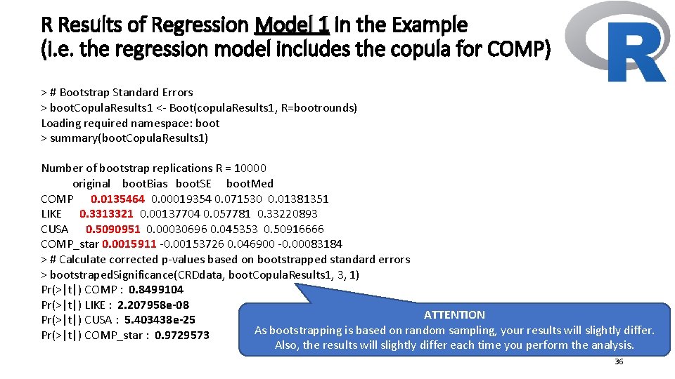
Prepare the R Code (IV) # Set bootstrapping rounds # FOR TESTING PURPOSE, WE RECOMMEND SETTING THIS VALUE TO 100; FOR REPORTING THE FINAL # RESULTS WE RECOMMEND SETTING IT TO 10000 bootrounds = 10000 Set the number of bootstraps (e. g. , 10, 000) # Calculate Results # Include Copula for COMP (Model 1) Run the regression model which includes the Gaussian copula for COMP # Normal regression copula. Results 1 <- lm (CUSL ~ COMP + LIKE + CUSA + COMP_star + 0) summary(copula. Results 1) # Bootstrap Standard Errors boot. Copula. Results 1 <- Boot(copula. Results 1, R=bootrounds) summary(boot. Copula. Results 1) # Calculate corrected p-values based on bootstrapped standard errors bootstraped. Significance(CRDdata, boot. Copula. Results 1, 3, 1) CHECK / UPDATE VALUES! 3 = Number of independent variables in the regression model 1 = Number of Gaussian copulas in the regression model 30

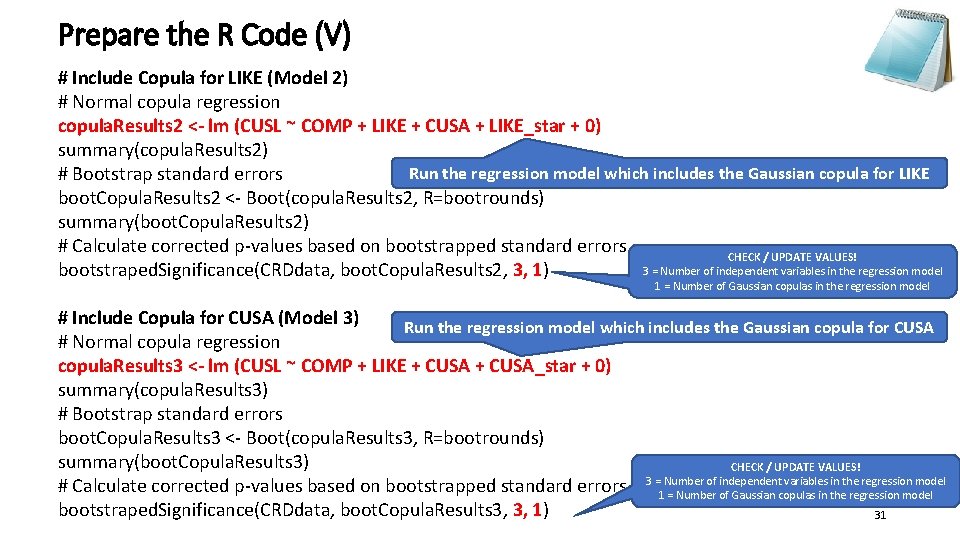
Prepare the R Code (V) # Include Copula for LIKE (Model 2) # Normal copula regression copula. Results 2 <- lm (CUSL ~ COMP + LIKE + CUSA + LIKE_star + 0) summary(copula. Results 2) Run the regression model which includes the Gaussian copula for LIKE # Bootstrap standard errors boot. Copula. Results 2 <- Boot(copula. Results 2, R=bootrounds) summary(boot. Copula. Results 2) # Calculate corrected p-values based on bootstrapped standard errors CHECK / UPDATE VALUES! 3 = Number of independent variables in the regression model bootstraped. Significance(CRDdata, boot. Copula. Results 2, 3, 1) 1 = Number of Gaussian copulas in the regression model # Include Copula for CUSA (Model 3) Run the regression model which includes the Gaussian copula for CUSA # Normal copula regression copula. Results 3 <- lm (CUSL ~ COMP + LIKE + CUSA_star + 0) summary(copula. Results 3) # Bootstrap standard errors boot. Copula. Results 3 <- Boot(copula. Results 3, R=bootrounds) summary(boot. Copula. Results 3) CHECK / UPDATE VALUES! of independent variables in the regression model # Calculate corrected p-values based on bootstrapped standard errors 3 =1 Number = Number of Gaussian copulas in the regression model bootstraped. Significance(CRDdata, boot. Copula. Results 3, 3, 1) 31

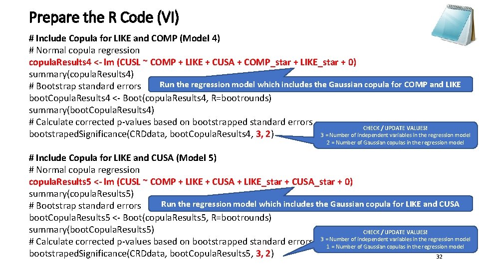
Prepare the R Code (VI) # Include Copula for LIKE and COMP (Model 4) # Normal copula regression copula. Results 4 <- lm (CUSL ~ COMP + LIKE + CUSA + COMP_star + LIKE_star + 0) summary(copula. Results 4) Run the regression model which includes the Gaussian copula for COMP and LIKE # Bootstrap standard errors boot. Copula. Results 4 <- Boot(copula. Results 4, R=bootrounds) summary(boot. Copula. Results 4) # Calculate corrected p-values based on bootstrapped standard errors CHECK / UPDATE VALUES! bootstraped. Significance(CRDdata, boot. Copula. Results 4, 3, 2) 3 = Number of independent variables in the regression model 2 = Number of Gaussian copulas in the regression model # Include Copula for LIKE and CUSA (Model 5) # Normal copula regression copula. Results 5 <- lm (CUSL ~ COMP + LIKE + CUSA + LIKE_star + CUSA_star + 0) summary(copula. Results 5) Run the regression model which includes the Gaussian copula for LIKE and CUSA # Bootstrap standard errors boot. Copula. Results 5 <- Boot(copula. Results 5, R=bootrounds) summary(boot. Copula. Results 5) CHECK / UPDATE VALUES! of independent variables in the regression model # Calculate corrected p-values based on bootstrapped standard errors 3 =1 Number = Number of Gaussian copulas in the regression model bootstraped. Significance(CRDdata, boot. Copula. Results 5, 3, 2) 32

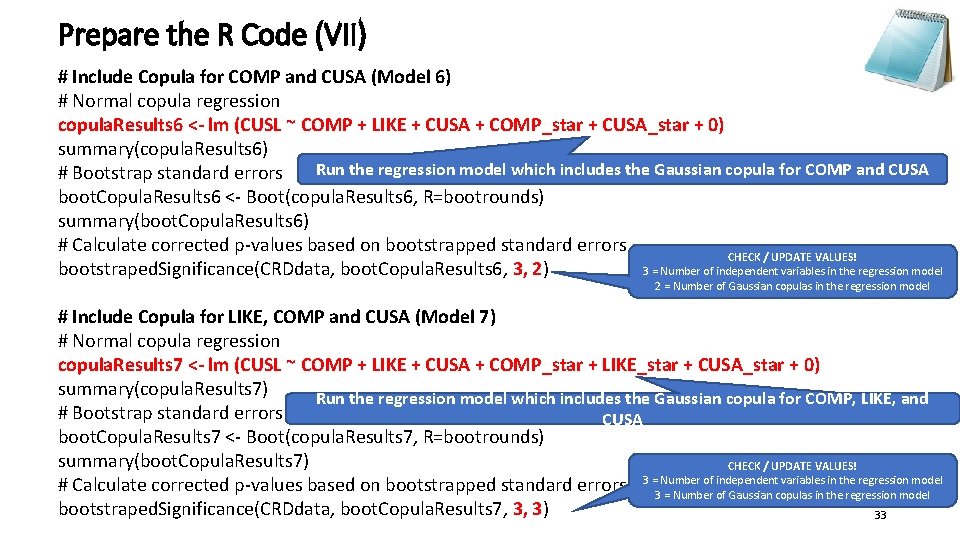
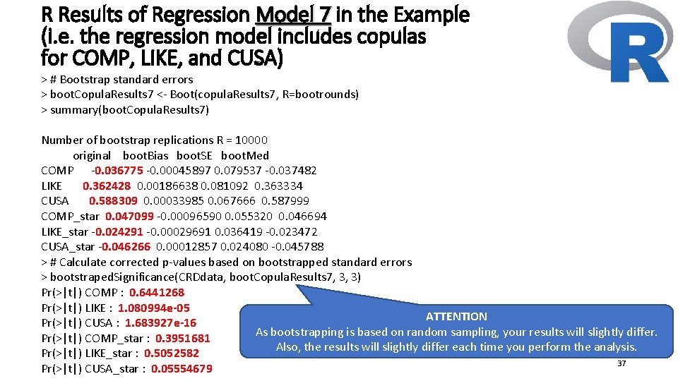
Prepare the R Code (VII) # Include Copula for COMP and CUSA (Model 6) # Normal copula regression copula. Results 6 <- lm (CUSL ~ COMP + LIKE + CUSA + COMP_star + CUSA_star + 0) summary(copula. Results 6) Run the regression model which includes the Gaussian copula for COMP and CUSA # Bootstrap standard errors boot. Copula. Results 6 <- Boot(copula. Results 6, R=bootrounds) summary(boot. Copula. Results 6) # Calculate corrected p-values based on bootstrapped standard errors CHECK / UPDATE VALUES! bootstraped. Significance(CRDdata, boot. Copula. Results 6, 3, 2) 3 = Number of independent variables in the regression model 2 = Number of Gaussian copulas in the regression model # Include Copula for LIKE, COMP and CUSA (Model 7) # Normal copula regression copula. Results 7 <- lm (CUSL ~ COMP + LIKE + CUSA + COMP_star + LIKE_star + CUSA_star + 0) summary(copula. Results 7) Run the regression model which includes the Gaussian copula for COMP, LIKE, and # Bootstrap standard errors CUSA boot. Copula. Results 7 <- Boot(copula. Results 7, R=bootrounds) summary(boot. Copula. Results 7) CHECK / UPDATE VALUES! of independent variables in the regression model # Calculate corrected p-values based on bootstrapped standard errors 3 =3 Number = Number of Gaussian copulas in the regression model bootstraped. Significance(CRDdata, boot. Copula. Results 7, 3, 3) 33

Create and estimate the PLS path model Data Preparation Generate the data file Prepare the R code for the requirements check Requirements Check Run the requirements check in R and analyze the results Model Analysis Prepare the R code for the Gaussian copula analysis Run the Gaussian copula analysis in R and interpret the results 34

Run R and Copy & Paste the Code Into the Console 35

R Results of Regression Model 1 in the Example (i. e. the regression model includes the copula for COMP) > # Bootstrap Standard Errors > boot. Copula. Results 1 <- Boot(copula. Results 1, R=bootrounds) Loading required namespace: boot > summary(boot. Copula. Results 1) Number of bootstrap replications R = 10000 original boot. Bias boot. SE boot. Med COMP 0. 0135464 0. 00019354 0. 071530 0. 01381351 LIKE 0. 3313321 0. 00137704 0. 057781 0. 33220893 CUSA 0. 5090951 0. 00030696 0. 045353 0. 50916666 COMP_star 0. 0015911 -0. 00153726 0. 046900 -0. 00083184 > # Calculate corrected p-values based on bootstrapped standard errors > bootstraped. Significance(CRDdata, boot. Copula. Results 1, 3, 1) Pr(>|t|) COMP : 0. 8499104 Pr(>|t|) LIKE : 2. 207958 e-08 ATTENTION Pr(>|t|) CUSA : 5. 403438 e-25 As bootstrapping is based on random sampling, your results will slightly differ. Pr(>|t|) COMP_star : 0. 9729573 Also, the results will slightly differ each time you perform the analysis. 36

R Results of Regression Model 7 in the Example (i. e. the regression model includes copulas for COMP, LIKE, and CUSA) > # Bootstrap standard errors > boot. Copula. Results 7 <- Boot(copula. Results 7, R=bootrounds) > summary(boot. Copula. Results 7) Number of bootstrap replications R = 10000 original boot. Bias boot. SE boot. Med COMP -0. 036775 -0. 00045897 0. 079537 -0. 037482 LIKE 0. 362428 0. 00186638 0. 081092 0. 363334 CUSA 0. 588309 0. 00033985 0. 067666 0. 587999 COMP_star 0. 047099 -0. 00096590 0. 055320 0. 046694 LIKE_star -0. 024291 -0. 00029691 0. 036419 -0. 023472 CUSA_star -0. 046266 0. 00012857 0. 024080 -0. 045788 > # Calculate corrected p-values based on bootstrapped standard errors > bootstraped. Significance(CRDdata, boot. Copula. Results 7, 3, 3) Pr(>|t|) COMP : 0. 6441268 Pr(>|t|) LIKE : 1. 080994 e-05 ATTENTION Pr(>|t|) CUSA : 1. 683927 e-16 As bootstrapping is based on random sampling, your results will slightly differ. Pr(>|t|) COMP_star : 0. 3951681 Also, the results will slightly differ each time you perform the analysis. Pr(>|t|) LIKE_star : 0. 5052582 37 Pr(>|t|) CUSA_star : 0. 05554679

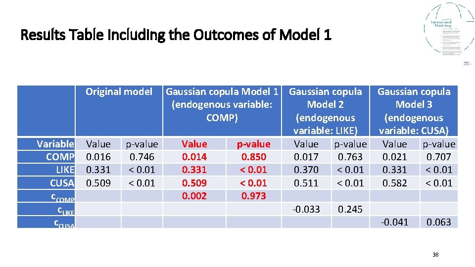
Results Table Including the Outcomes of Model 1 Original model Variable COMP LIKE CUSA c. COMP c. LIKE c. CUSA Value 0. 016 0. 331 0. 509 Gaussian copula Model 1 Gaussian copula (endogenous variable: Model 2 Model 3 COMP) (endogenous variable: LIKE) variable: CUSA) p-value Value p-value 0. 746 0. 014 0. 850 0. 017 0. 763 0. 021 0. 707 < 0. 01 0. 331 < 0. 01 0. 370 < 0. 01 0. 331 < 0. 01 0. 509 < 0. 01 0. 511 < 0. 01 0. 582 < 0. 01 0. 002 0. 973 -0. 033 0. 245 -0. 041 0. 063 38

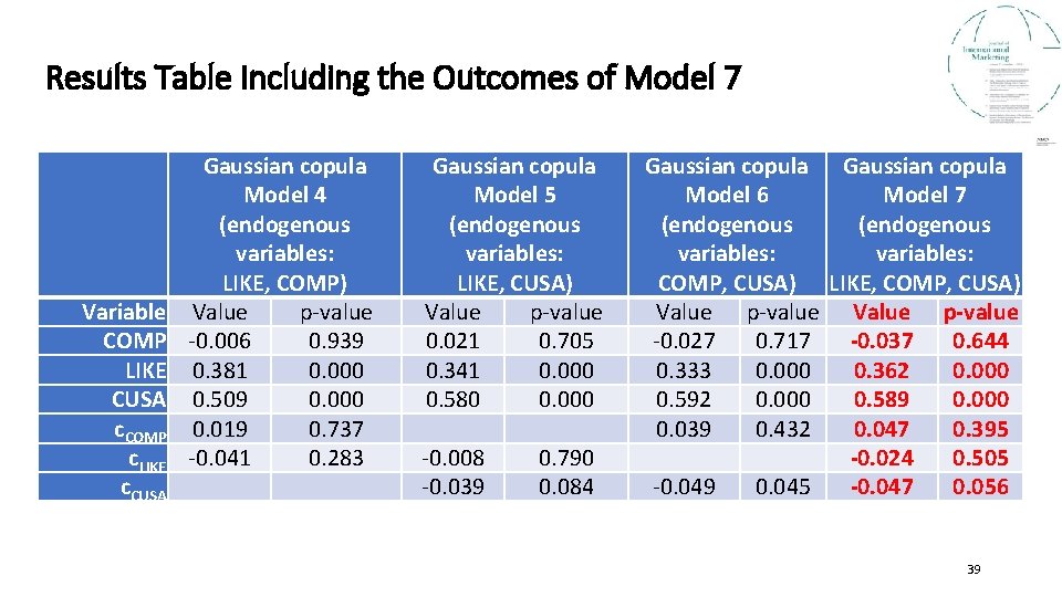
Results Table Including the Outcomes of Model 7 Variable COMP LIKE CUSA c. COMP c. LIKE c. CUSA Gaussian copula Model 4 (endogenous variables: LIKE, COMP) Value p-value -0. 006 0. 939 0. 381 0. 000 0. 509 0. 000 0. 019 0. 737 -0. 041 0. 283 Gaussian copula Model 5 (endogenous variables: LIKE, CUSA) Value p-value 0. 021 0. 705 0. 341 0. 000 0. 580 0. 000 -0. 008 -0. 039 0. 790 0. 084 Gaussian copula Model 6 Model 7 (endogenous variables: COMP, CUSA) LIKE, COMP, CUSA) Value p-value -0. 027 0. 717 -0. 037 0. 644 0. 333 0. 000 0. 362 0. 000 0. 592 0. 000 0. 589 0. 000 0. 039 0. 432 0. 047 0. 395 -0. 024 0. 505 -0. 049 0. 045 -0. 047 0. 056 39

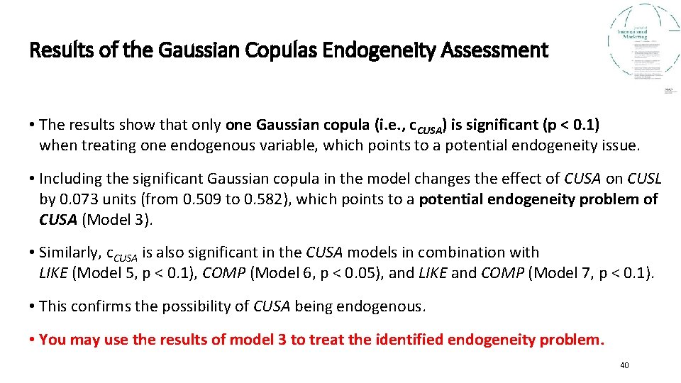
Results of the Gaussian Copulas Endogeneity Assessment • The results show that only one Gaussian copula (i. e. , c. CUSA) is significant (p < 0. 1) when treating one endogenous variable, which points to a potential endogeneity issue. • Including the significant Gaussian copula in the model changes the effect of CUSA on CUSL by 0. 073 units (from 0. 509 to 0. 582), which points to a potential endogeneity problem of CUSA (Model 3). • Similarly, c. CUSA is also significant in the CUSA models in combination with LIKE (Model 5, p < 0. 1), COMP (Model 6, p < 0. 05), and LIKE and COMP (Model 7, p < 0. 1). • This confirms the possibility of CUSA being endogenous. • You may use the results of model 3 to treat the identified endogeneity problem. 40

http: //journals. ama. org/doi/10. 1509/jim. 17. 0151 Further Research? Hult, G. T. M. , J. F. Hair, D. Proksch, M. Sarstedt, A. Pinkwart, & C. M. Ringle (2018). Addressing Endogeneity in International Marketing Applications of Partial Least Squares Structural Equation Modeling. Journal of International Marketing, forthcoming. 41

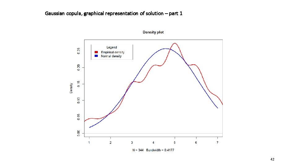
Gaussian copula, graphical representation of solution – part 1 42

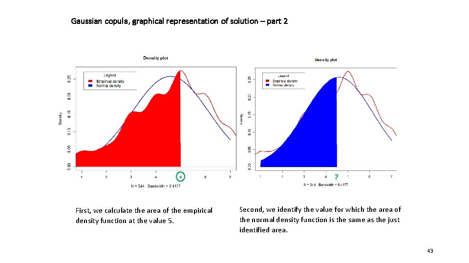
Gaussian copula, graphical representation of solution – part 2 ? First, we calculate the area of the empirical density function at the value 5. Second, we identify the value for which the area of the normal density function is the same as the just identified area. 43

Explanation of Gaussian Copula approach – Part 1 44

Explanation of Gaussian Copula approach – Part 2 45