ECE 6504 Deep Learning for Perception Topics Finish

ECE 6504: Deep Learning for Perception Topics: – (Finish) Backprop – Convolutional Neural Nets Dhruv Batra Virginia Tech

Administrativia • Presentation Assignments – https: //docs. google. com/spreadsheets/d/1 m 76 E 4 m. C 0 wf. Rjc 4 HRBWFd. Al. XKPIzl. Ewfw 1 -u 7 r. Bw 9 TJ 8/edit#gid=2045905312 (C) Dhruv Batra 2

Recap of last time (C) Dhruv Batra 3

Last Time • Notation + Setup • Neural Networks • Chain Rule + Backprop (C) Dhruv Batra 4

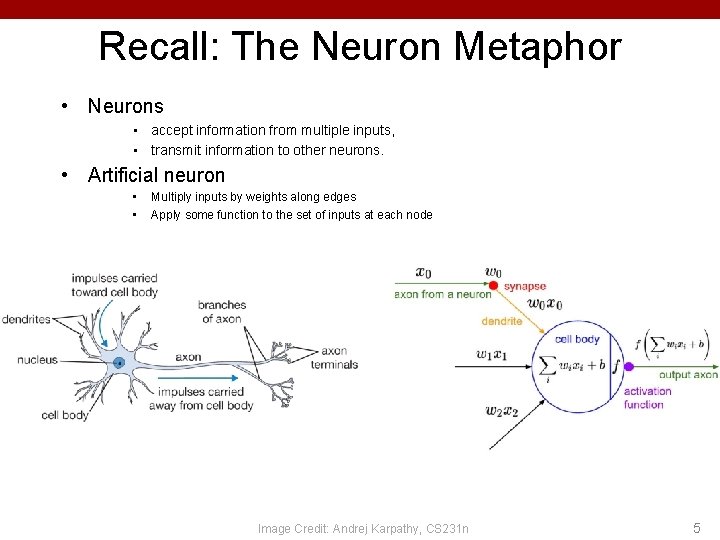
Recall: The Neuron Metaphor • Neurons • accept information from multiple inputs, • transmit information to other neurons. • Artificial neuron • • Multiply inputs by weights along edges Apply some function to the set of inputs at each node Image Credit: Andrej Karpathy, CS 231 n 5

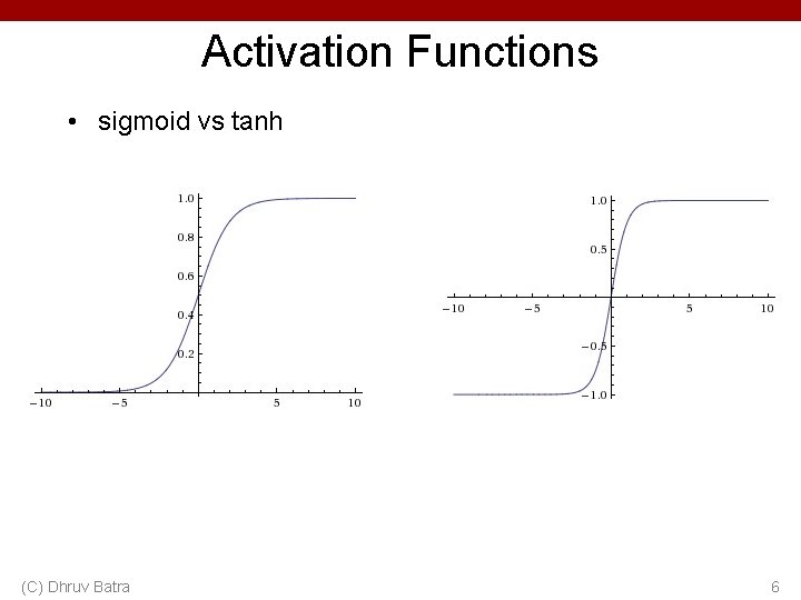
Activation Functions • sigmoid vs tanh (C) Dhruv Batra 6

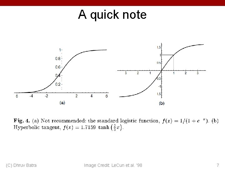
A quick note (C) Dhruv Batra Image Credit: Le. Cun et al. ‘ 98 7

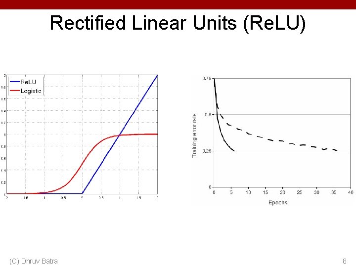
Rectified Linear Units (Re. LU) (C) Dhruv Batra 8

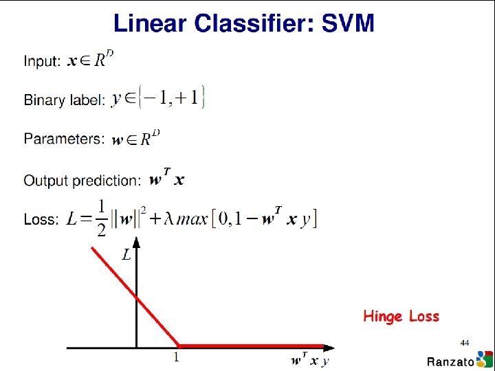
(C) Dhruv Batra 9

(C) Dhruv Batra 10

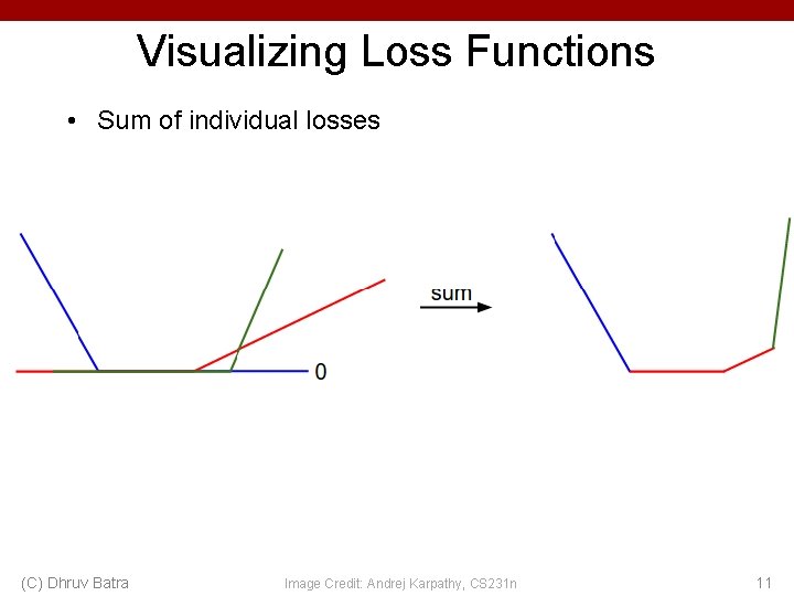
Visualizing Loss Functions • Sum of individual losses (C) Dhruv Batra Image Credit: Andrej Karpathy, CS 231 n 11

Detour (C) Dhruv Batra 12

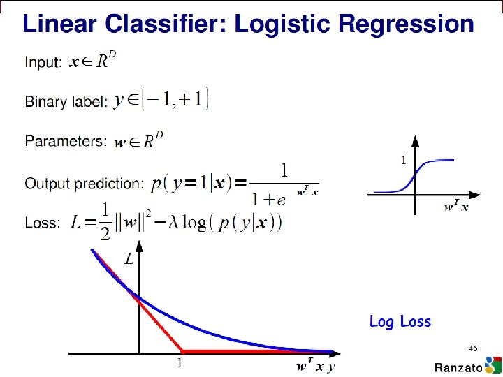
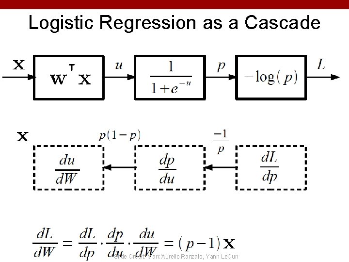
Logistic Regression as a Cascade (C) Dhruv Batra Slide Credit: Marc'Aurelio Ranzato, Yann Le. Cun 13

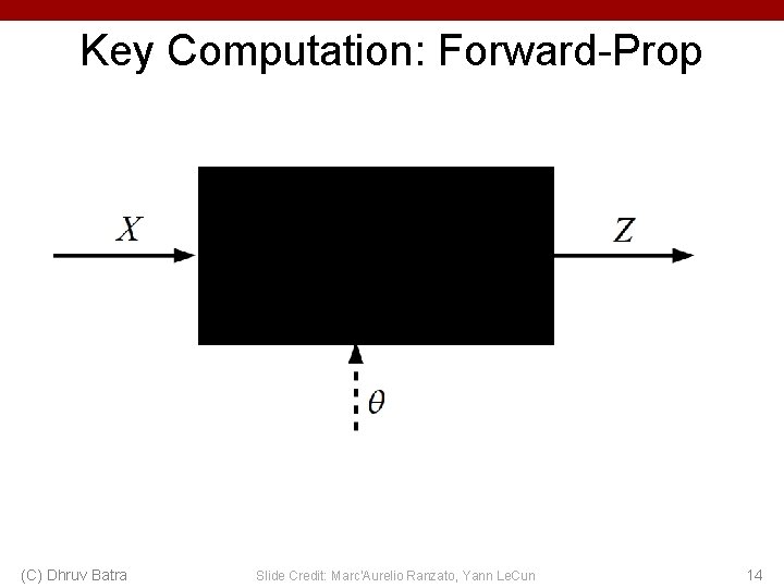
Key Computation: Forward-Prop (C) Dhruv Batra Slide Credit: Marc'Aurelio Ranzato, Yann Le. Cun 14

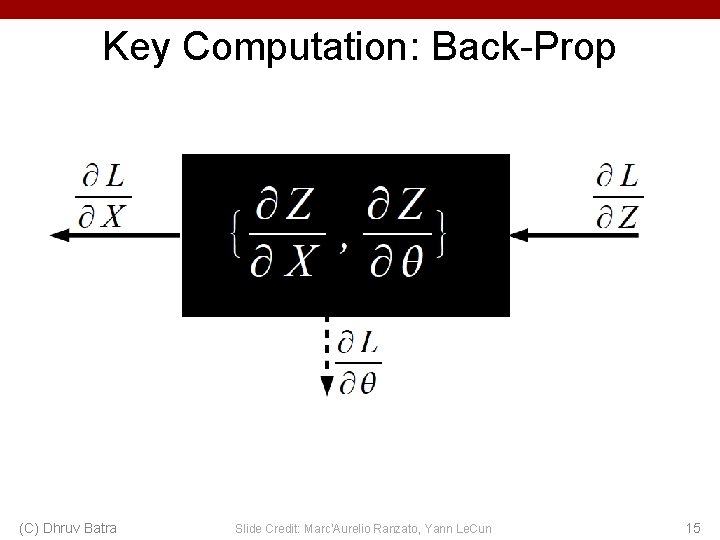
Key Computation: Back-Prop (C) Dhruv Batra Slide Credit: Marc'Aurelio Ranzato, Yann Le. Cun 15

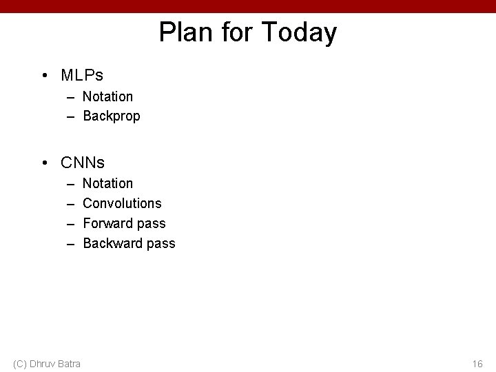
Plan for Today • MLPs – Notation – Backprop • CNNs – – (C) Dhruv Batra Notation Convolutions Forward pass Backward pass 16

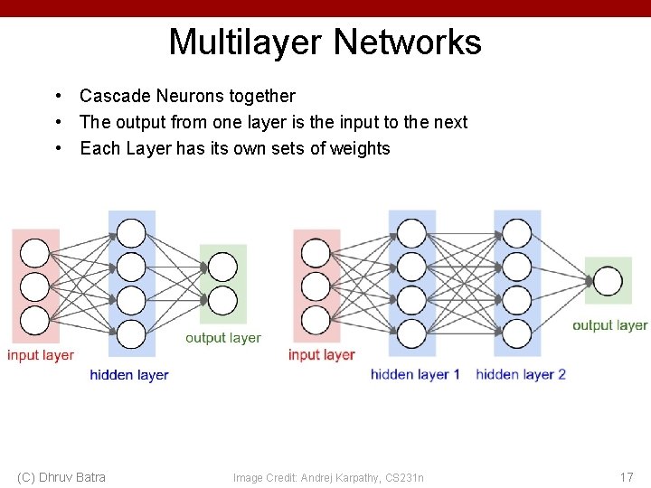
Multilayer Networks • Cascade Neurons together • The output from one layer is the input to the next • Each Layer has its own sets of weights (C) Dhruv Batra Image Credit: Andrej Karpathy, CS 231 n 17

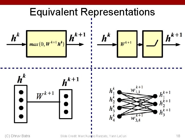
Equivalent Representations (C) Dhruv Batra Slide Credit: Marc'Aurelio Ranzato, Yann Le. Cun 18

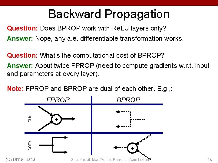
Backward Propagation Question: Does BPROP work with Re. LU layers only? Answer: Nope, any a. e. differentiable transformation works. Question: What's the computational cost of BPROP? Answer: About twice FPROP (need to compute gradients w. r. t. input and parameters at every layer). Note: FPROP and BPROP are dual of each other. E. g. , : COPY SUM FPROP (C) Dhruv Batra BPROP + + Slide Credit: Marc'Aurelio Ranzato, Yann Le. Cun 19

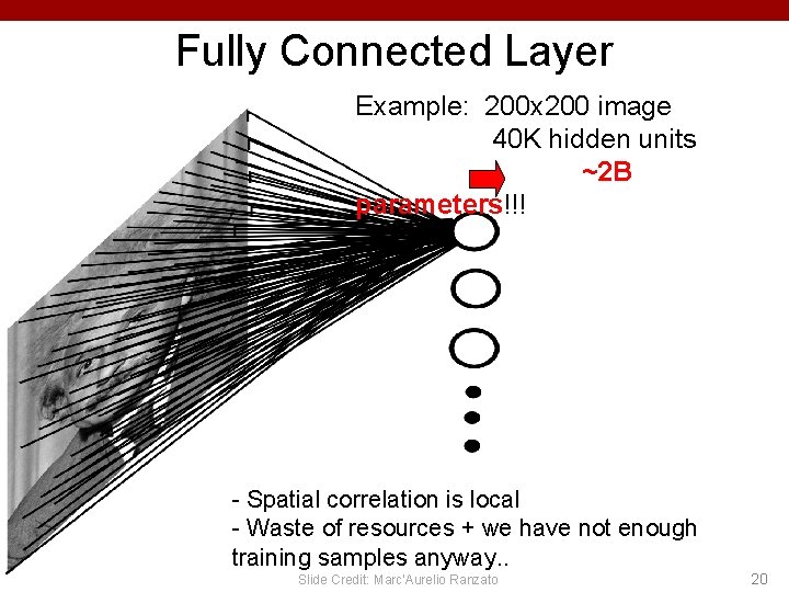
Fully Connected Layer Example: 200 x 200 image 40 K hidden units ~2 B parameters!!! - Spatial correlation is local - Waste of resources + we have not enough training samples anyway. . Slide Credit: Marc'Aurelio Ranzato 20

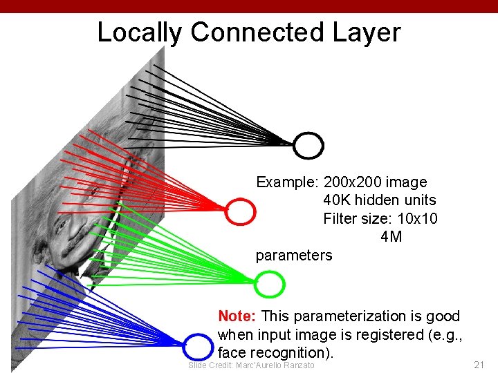
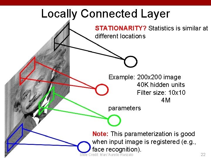
Locally Connected Layer Example: 200 x 200 image 40 K hidden units Filter size: 10 x 10 4 M parameters Note: This parameterization is good when input image is registered (e. g. , face recognition). Slide Credit: Marc'Aurelio Ranzato 21

Locally Connected Layer STATIONARITY? Statistics is similar at different locations Example: 200 x 200 image 40 K hidden units Filter size: 10 x 10 4 M parameters Note: This parameterization is good when input image is registered (e. g. , face recognition). Slide Credit: Marc'Aurelio Ranzato 22

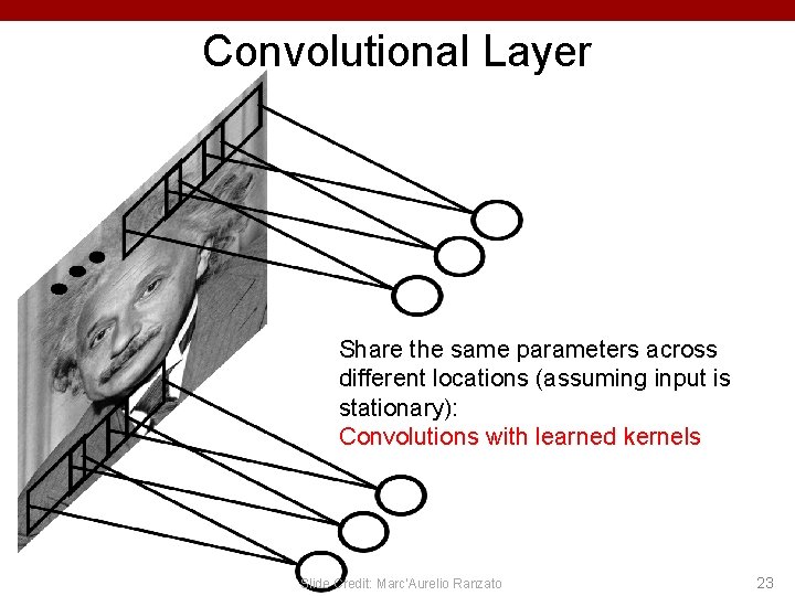
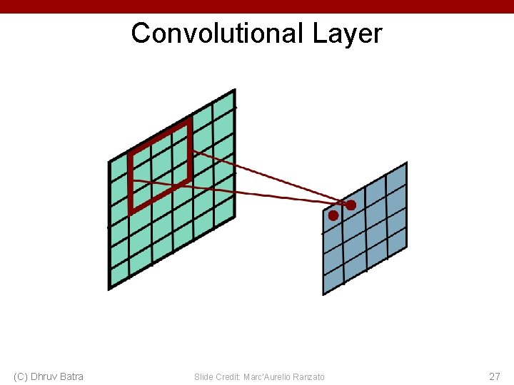
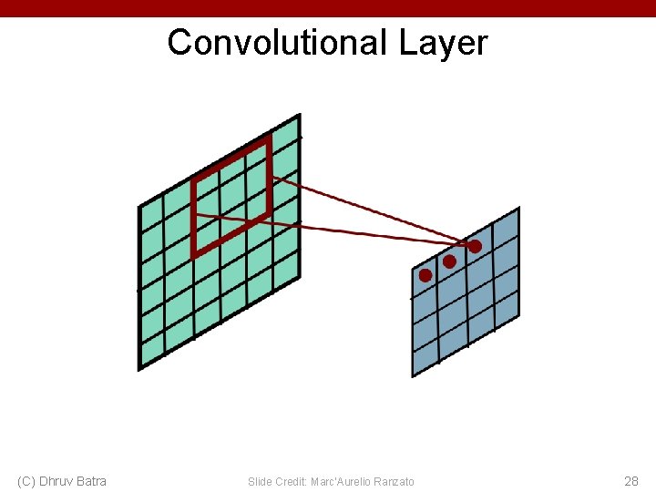
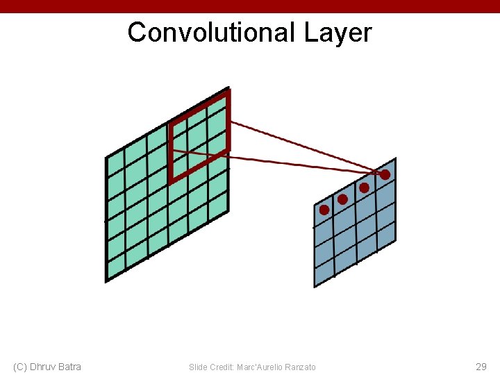
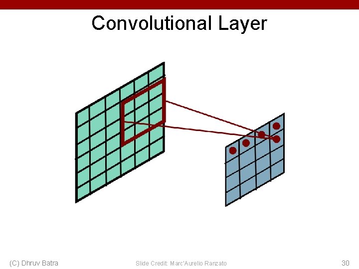
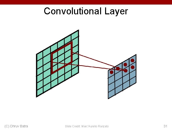
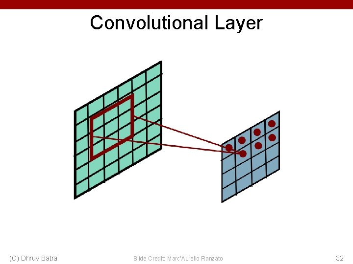
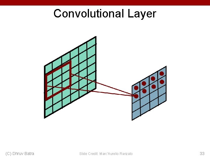
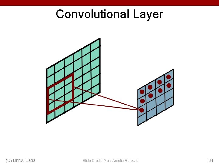
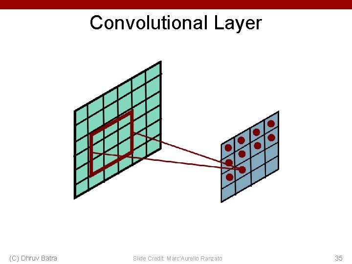
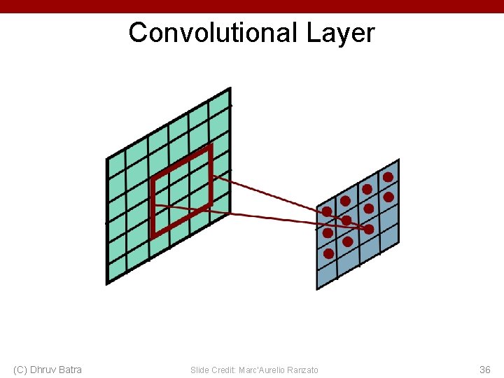
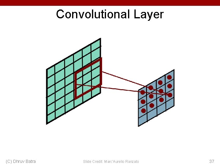
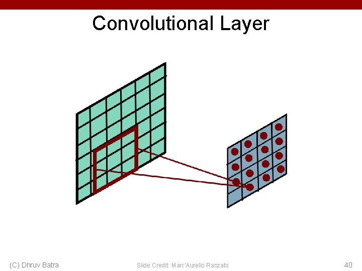
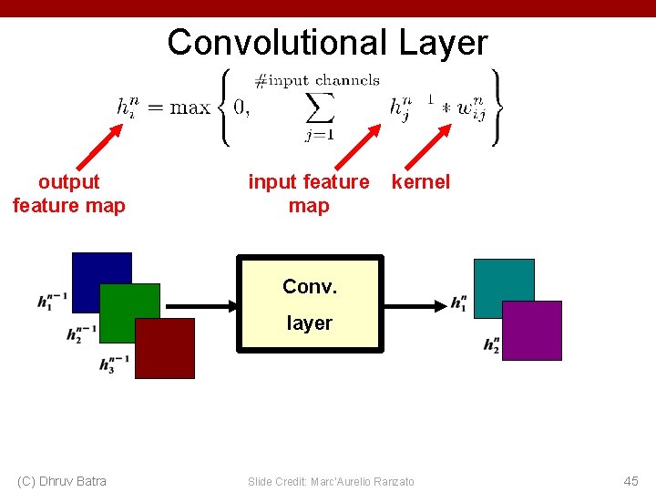
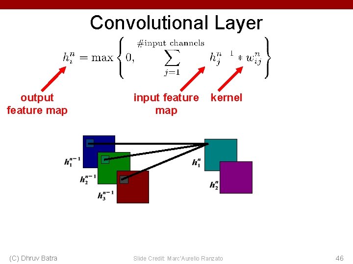
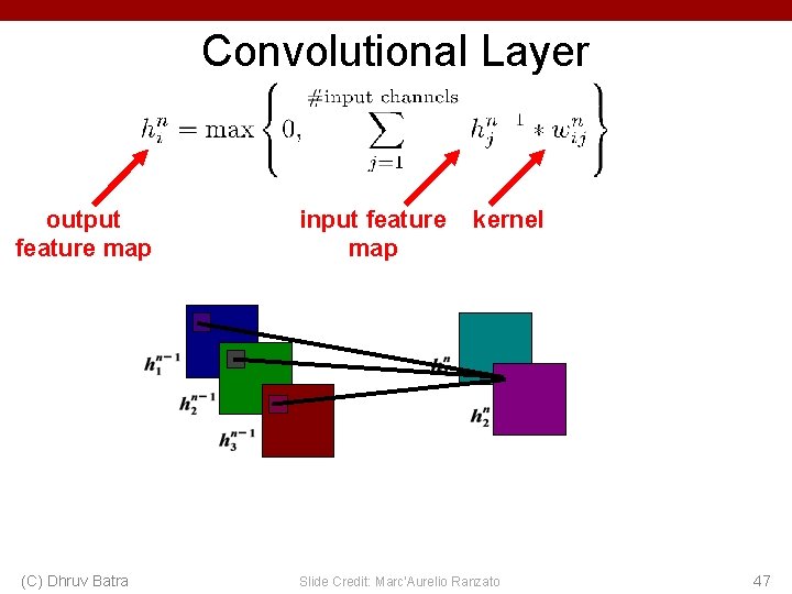
Convolutional Layer Share the same parameters across different locations (assuming input is stationary): Convolutions with learned kernels Slide Credit: Marc'Aurelio Ranzato 23

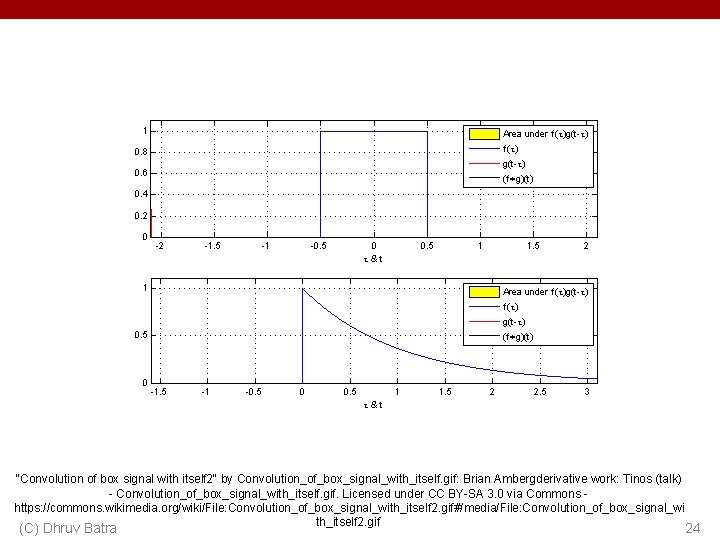
"Convolution of box signal with itself 2" by Convolution_of_box_signal_with_itself. gif: Brian Ambergderivative work: Tinos (talk) - Convolution_of_box_signal_with_itself. gif. Licensed under CC BY-SA 3. 0 via Commons https: //commons. wikimedia. org/wiki/File: Convolution_of_box_signal_with_itself 2. gif#/media/File: Convolution_of_box_signal_wi th_itself 2. gif (C) Dhruv Batra 24

Convolution Explained • http: //setosa. io/ev/image-kernels/ • https: //github. com/bruckner/deep. Viz (C) Dhruv Batra 25

Convolutional Layer (C) Dhruv Batra Slide Credit: Marc'Aurelio Ranzato 26

Convolutional Layer (C) Dhruv Batra Slide Credit: Marc'Aurelio Ranzato 27

Convolutional Layer (C) Dhruv Batra Slide Credit: Marc'Aurelio Ranzato 28

Convolutional Layer (C) Dhruv Batra Slide Credit: Marc'Aurelio Ranzato 29

Convolutional Layer (C) Dhruv Batra Slide Credit: Marc'Aurelio Ranzato 30

Convolutional Layer (C) Dhruv Batra Slide Credit: Marc'Aurelio Ranzato 31

Convolutional Layer (C) Dhruv Batra Slide Credit: Marc'Aurelio Ranzato 32

Convolutional Layer (C) Dhruv Batra Slide Credit: Marc'Aurelio Ranzato 33

Convolutional Layer (C) Dhruv Batra Slide Credit: Marc'Aurelio Ranzato 34

Convolutional Layer (C) Dhruv Batra Slide Credit: Marc'Aurelio Ranzato 35

Convolutional Layer (C) Dhruv Batra Slide Credit: Marc'Aurelio Ranzato 36

Convolutional Layer (C) Dhruv Batra Slide Credit: Marc'Aurelio Ranzato 37

Convolutional Layer (C) Dhruv Batra Slide Credit: Marc'Aurelio Ranzato 38

Convolutional Layer (C) Dhruv Batra Slide Credit: Marc'Aurelio Ranzato 39

Convolutional Layer (C) Dhruv Batra Slide Credit: Marc'Aurelio Ranzato 40

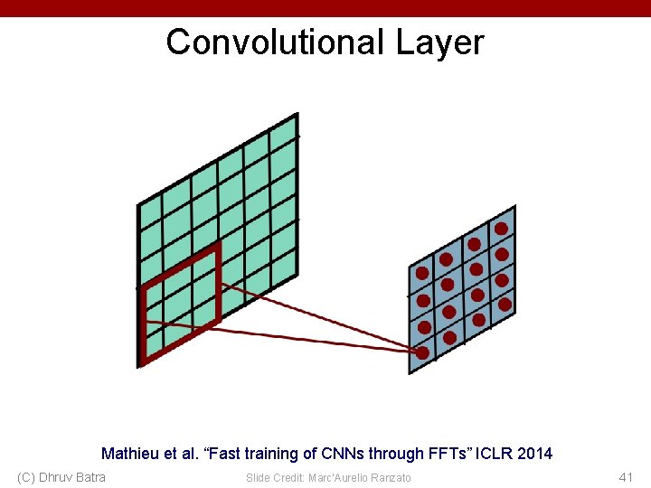
Convolutional Layer Mathieu et al. “Fast training of CNNs through FFTs” ICLR 2014 (C) Dhruv Batra Slide Credit: Marc'Aurelio Ranzato 41

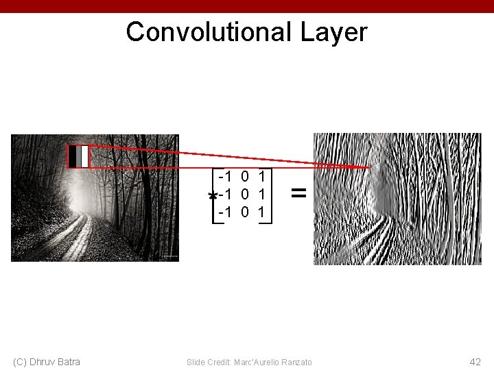
Convolutional Layer * (C) Dhruv Batra -1 0 1 = Slide Credit: Marc'Aurelio Ranzato 42

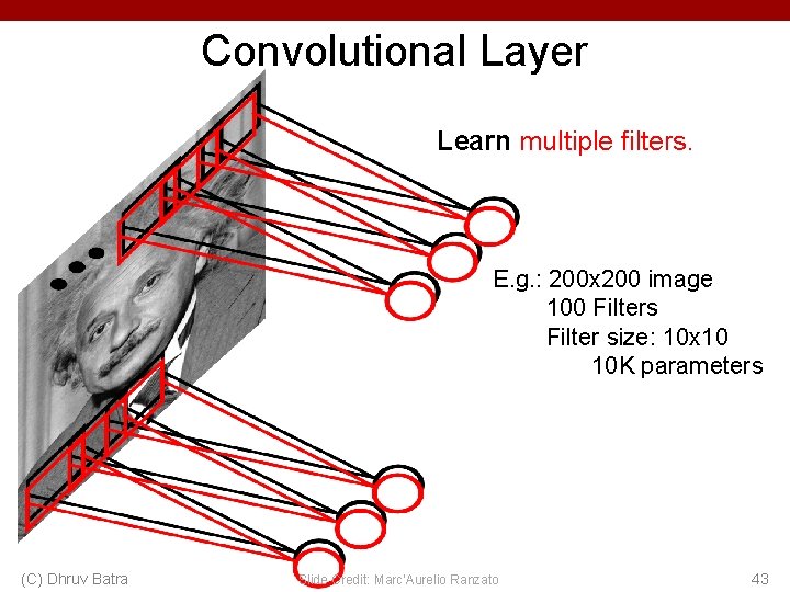
Convolutional Layer Learn multiple filters. E. g. : 200 x 200 image 100 Filters Filter size: 10 x 10 10 K parameters (C) Dhruv Batra Slide Credit: Marc'Aurelio Ranzato 43

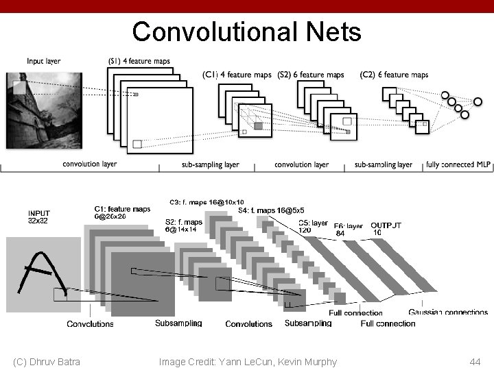
Convolutional Nets a (C) Dhruv Batra Image Credit: Yann Le. Cun, Kevin Murphy 44

Convolutional Layer output feature map input feature map kernel Conv. layer (C) Dhruv Batra Slide Credit: Marc'Aurelio Ranzato 45

Convolutional Layer output feature map (C) Dhruv Batra input feature map kernel Slide Credit: Marc'Aurelio Ranzato 46

Convolutional Layer output feature map (C) Dhruv Batra input feature map kernel Slide Credit: Marc'Aurelio Ranzato 47

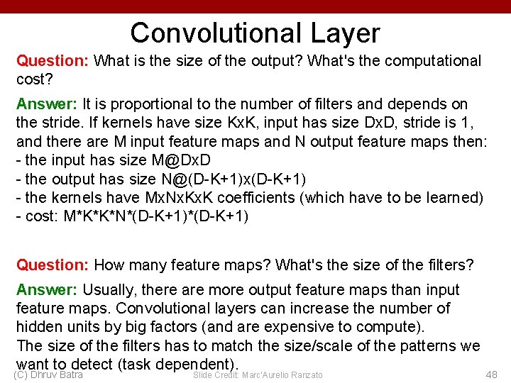
Convolutional Layer Question: What is the size of the output? What's the computational cost? Answer: It is proportional to the number of filters and depends on the stride. If kernels have size Kx. K, input has size Dx. D, stride is 1, and there are M input feature maps and N output feature maps then: - the input has size M@Dx. D - the output has size N@(D-K+1)x(D-K+1) - the kernels have Mx. Nx. K coefficients (which have to be learned) - cost: M*K*K*N*(D-K+1) Question: How many feature maps? What's the size of the filters? Answer: Usually, there are more output feature maps than input feature maps. Convolutional layers can increase the number of hidden units by big factors (and are expensive to compute). The size of the filters has to match the size/scale of the patterns we want to detect (task dependent). (C) Dhruv Batra Slide Credit: Marc'Aurelio Ranzato 48

Key Ideas A standard neural net applied to images: - scales quadratically with the size of the input - does not leverage stationarity Solution: - connect each hidden unit to a small patch of the input - share the weight across space This is called: convolutional layer. A network with convolutional layers is called convolutional network. Le. Cun et al. “Gradient-based learning applied to document recognition” IEEE 1998 (C) Dhruv Batra Slide Credit: Marc'Aurelio Ranzato 49

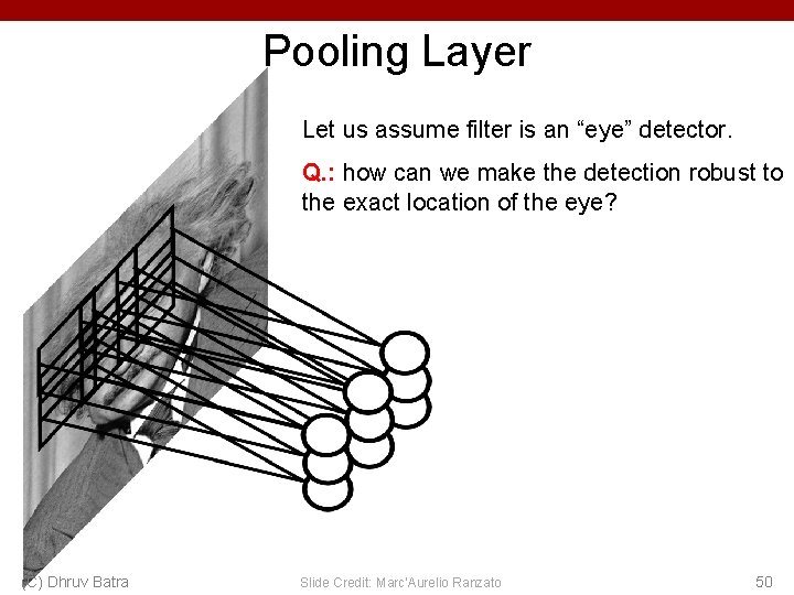
Pooling Layer Let us assume filter is an “eye” detector. Q. : how can we make the detection robust to the exact location of the eye? (C) Dhruv Batra Slide Credit: Marc'Aurelio Ranzato 50

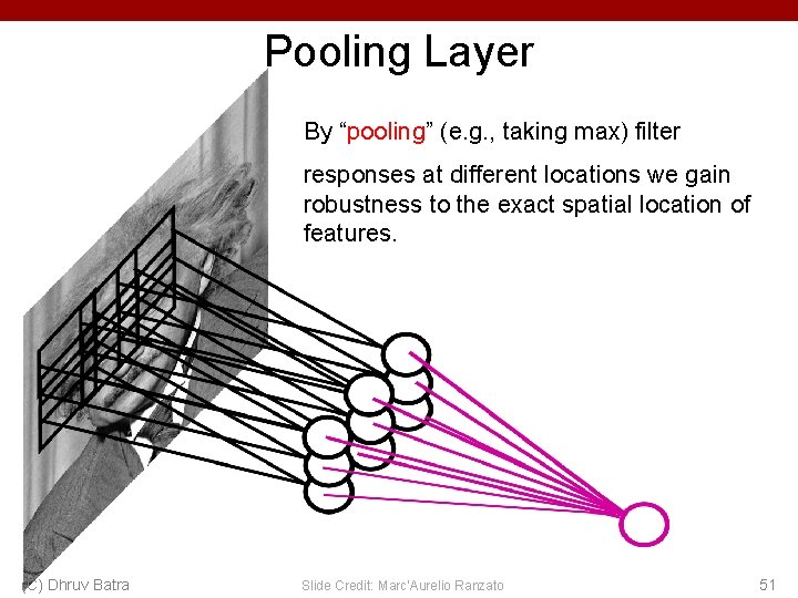
Pooling Layer By “pooling” (e. g. , taking max) filter responses at different locations we gain robustness to the exact spatial location of features. (C) Dhruv Batra Slide Credit: Marc'Aurelio Ranzato 51

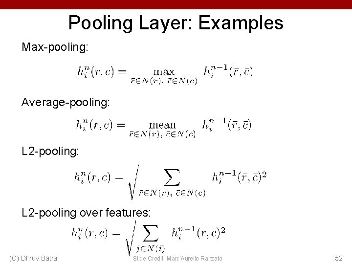
Pooling Layer: Examples Max-pooling: Average-pooling: L 2 -pooling over features: (C) Dhruv Batra Slide Credit: Marc'Aurelio Ranzato 52

Pooling Layer Question: What is the size of the output? What's the computational cost? Answer: The size of the output depends on the stride between the pools. For instance, if pools do not overlap and have size Kx. K, and the input has size Dx. D with M input feature maps, then: - output is M@(D/K)x(D/K) - the computational cost is proportional to the size of the input (negligible compared to a convolutional layer) Question: How should I set the size of the pools? Answer: It depends on how much “invariant” or robust to distortions we want the representation to be. It is best to pool slowly (via a few stacks of conv-pooling layers). (C) Dhruv Batra Slide Credit: Marc'Aurelio Ranzato 53

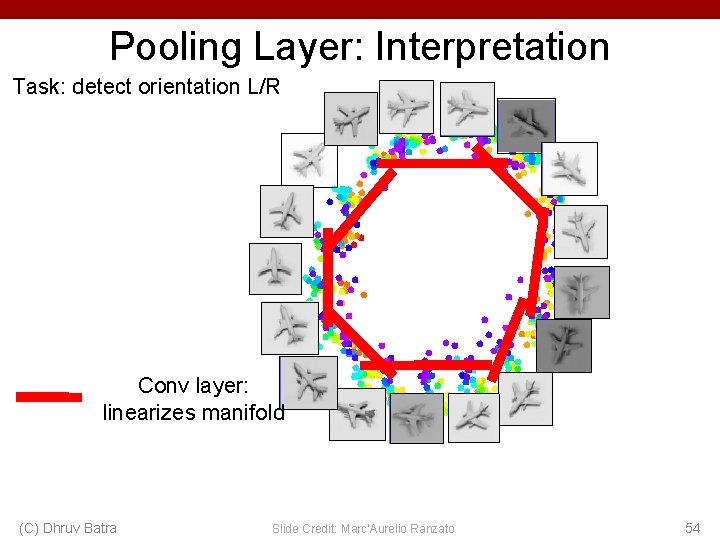
Pooling Layer: Interpretation Task: detect orientation L/R Conv layer: linearizes manifold (C) Dhruv Batra Slide Credit: Marc'Aurelio Ranzato 54

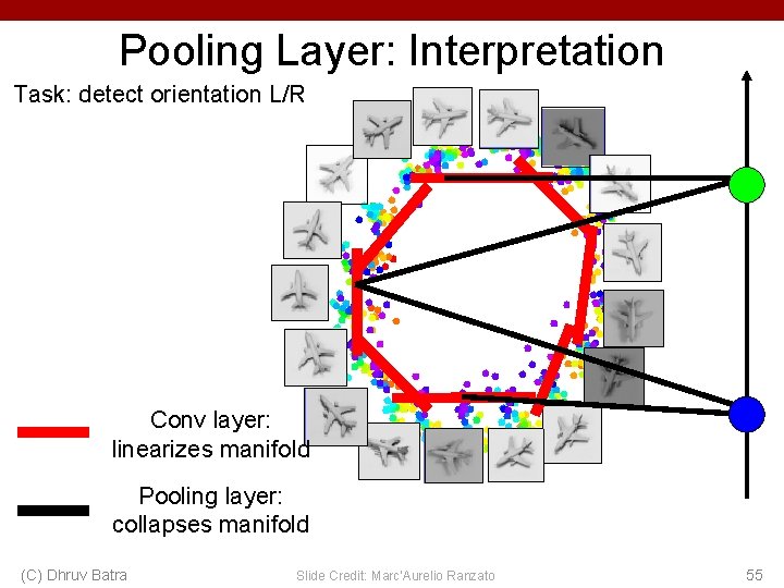
Pooling Layer: Interpretation Task: detect orientation L/R Conv layer: linearizes manifold Pooling layer: collapses manifold (C) Dhruv Batra Slide Credit: Marc'Aurelio Ranzato 55

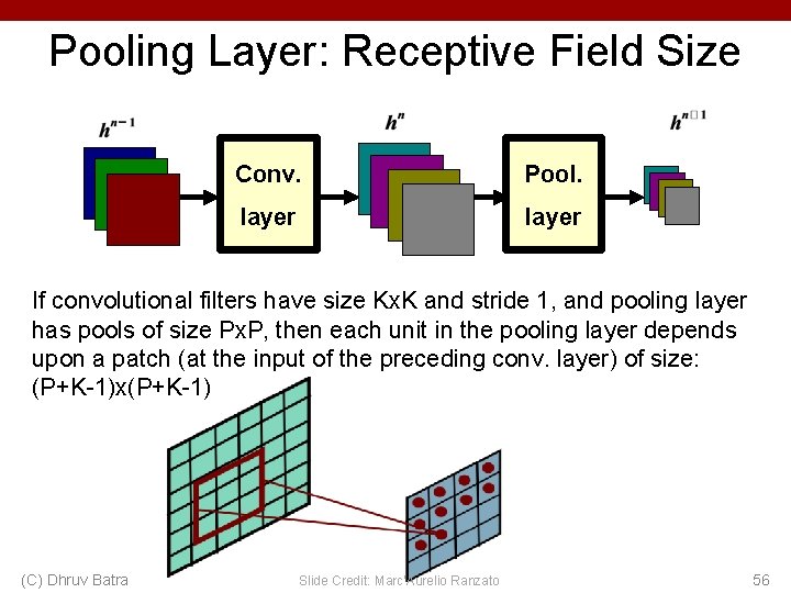
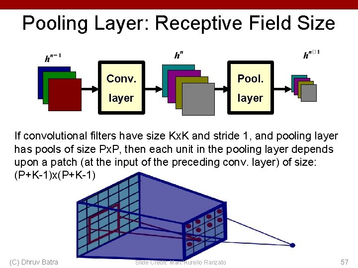
Pooling Layer: Receptive Field Size Conv. Pool. layer If convolutional filters have size Kx. K and stride 1, and pooling layer has pools of size Px. P, then each unit in the pooling layer depends upon a patch (at the input of the preceding conv. layer) of size: (P+K-1)x(P+K-1) (C) Dhruv Batra Slide Credit: Marc'Aurelio Ranzato 56

Pooling Layer: Receptive Field Size Conv. Pool. layer If convolutional filters have size Kx. K and stride 1, and pooling layer has pools of size Px. P, then each unit in the pooling layer depends upon a patch (at the input of the preceding conv. layer) of size: (P+K-1)x(P+K-1) (C) Dhruv Batra Slide Credit: Marc'Aurelio Ranzato 57

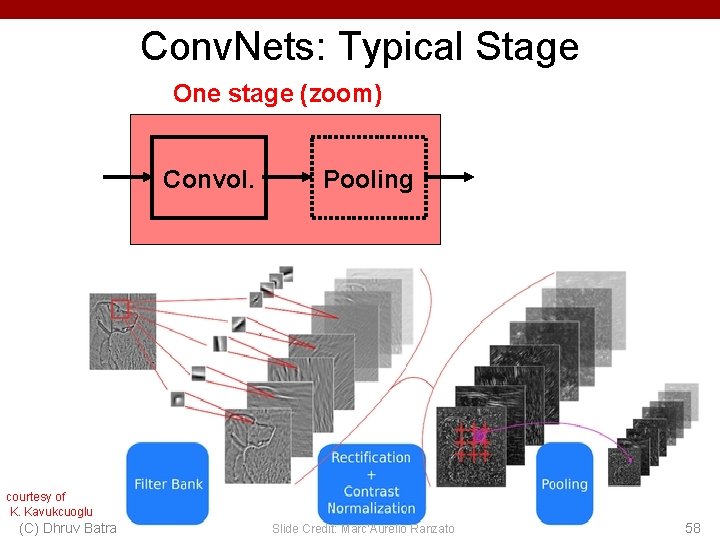
Conv. Nets: Typical Stage One stage (zoom) Convol. Pooling courtesy of K. Kavukcuoglu (C) Dhruv Batra Slide Credit: Marc'Aurelio Ranzato 58

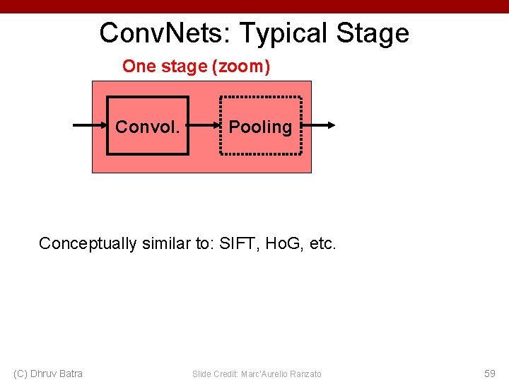
Conv. Nets: Typical Stage One stage (zoom) Convol. Pooling Conceptually similar to: SIFT, Ho. G, etc. (C) Dhruv Batra Slide Credit: Marc'Aurelio Ranzato 59

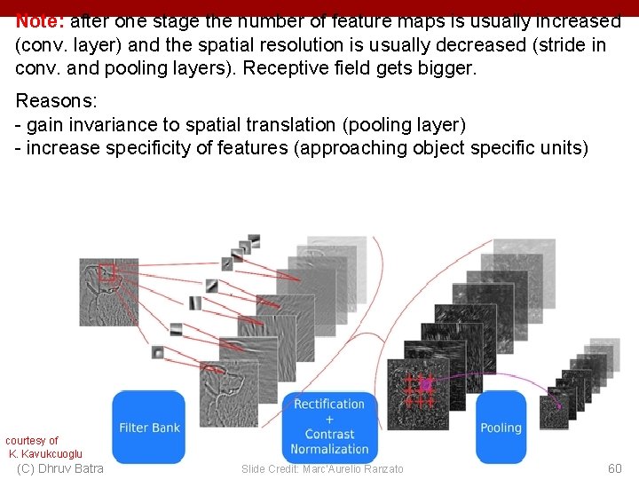
Note: after one stage the number of feature maps is usually increased (conv. layer) and the spatial resolution is usually decreased (stride in conv. and pooling layers). Receptive field gets bigger. Reasons: - gain invariance to spatial translation (pooling layer) - increase specificity of features (approaching object specific units) courtesy of K. Kavukcuoglu (C) Dhruv Batra Slide Credit: Marc'Aurelio Ranzato 60

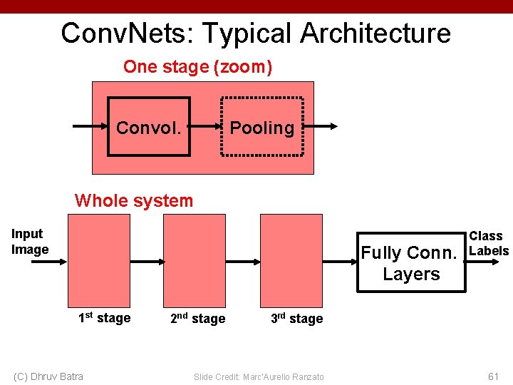
Conv. Nets: Typical Architecture One stage (zoom) Convol. Pooling Whole system Input Image Fully Conn. Layers 1 st stage (C) Dhruv Batra 2 nd stage Class Labels 3 rd stage Slide Credit: Marc'Aurelio Ranzato 61

Visualizing Learned Filters (C) Dhruv Batra Figure Credit: [Zeiler & Fergus ECCV 14] 62

Visualizing Learned Filters (C) Dhruv Batra Figure Credit: [Zeiler & Fergus ECCV 14] 63

Visualizing Learned Filters (C) Dhruv Batra Figure Credit: [Zeiler & Fergus ECCV 14] 64

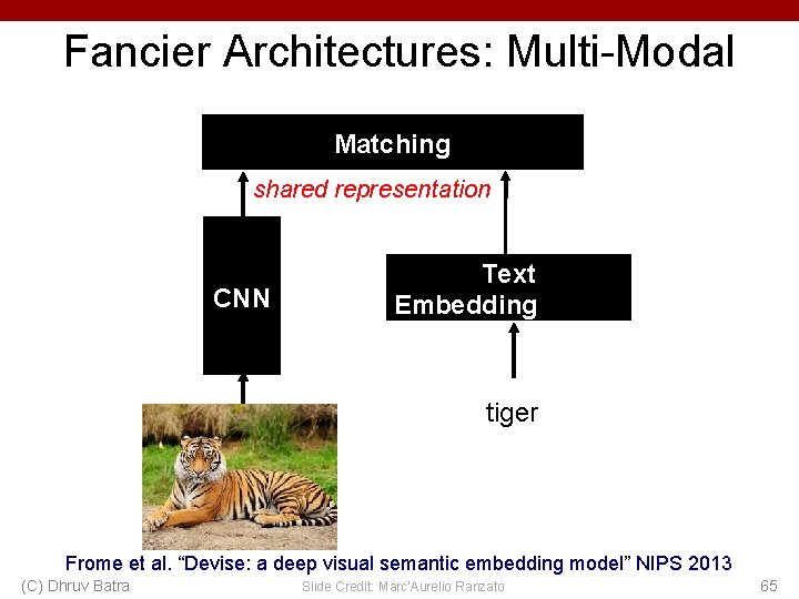
Fancier Architectures: Multi-Modal Matching shared representation CNN Text Embedding tiger Frome et al. “Devise: a deep visual semantic embedding model” NIPS 2013 (C) Dhruv Batra Slide Credit: Marc'Aurelio Ranzato 65

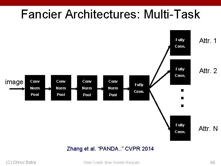
Fancier Architectures: Multi-Task Fully Conn. Fully image Conv Norm Pool Fully Conn. Attr. 2 . . . Conn. Attr. 1 Fully Conn. Attr. N Zhang et al. “PANDA. . ” CVPR 2014 (C) Dhruv Batra Slide Credit: Marc'Aurelio Ranzato 66

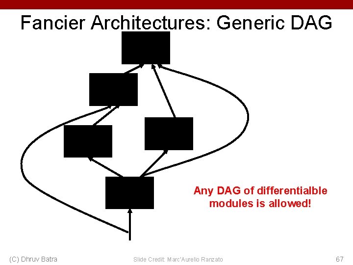
Fancier Architectures: Generic DAG Any DAG of differentialble modules is allowed! (C) Dhruv Batra Slide Credit: Marc'Aurelio Ranzato 67