ECE 6504 Deep Learning for Perception Topics Toeplitz

ECE 6504: Deep Learning for Perception Topics: – Toeplitz Matrix – 1 x 1 Convolution – AKA How to run a Conv. Net on arbitrary sized images Dhruv Batra Virginia Tech

Plan for Today • Toeplitz Matrix • 1 x 1 Convolution – AKA How to run a Conv. Net on arbitrary sized images (C) Dhruv Batra 2

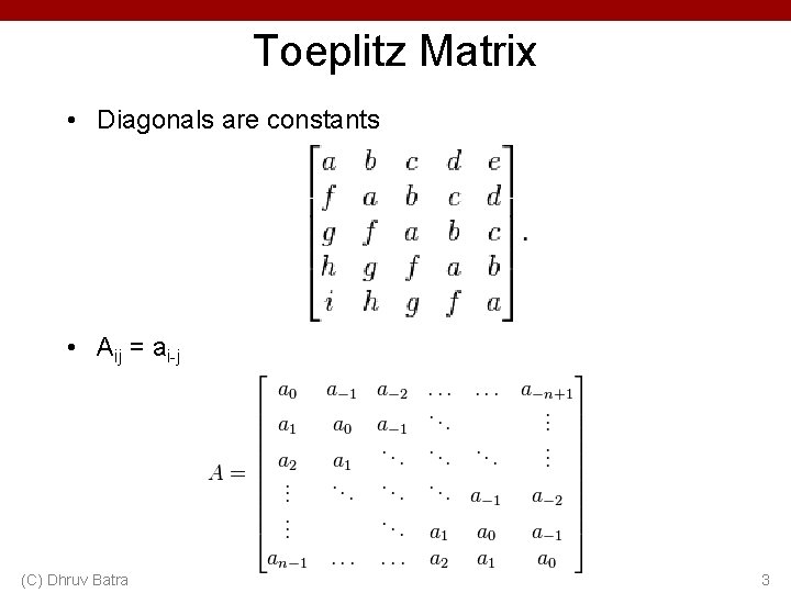
Toeplitz Matrix • Diagonals are constants • Aij = ai-j (C) Dhruv Batra 3

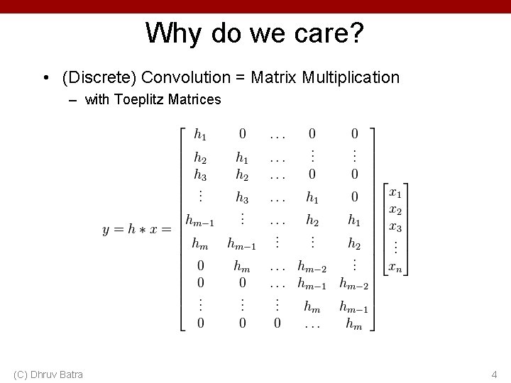
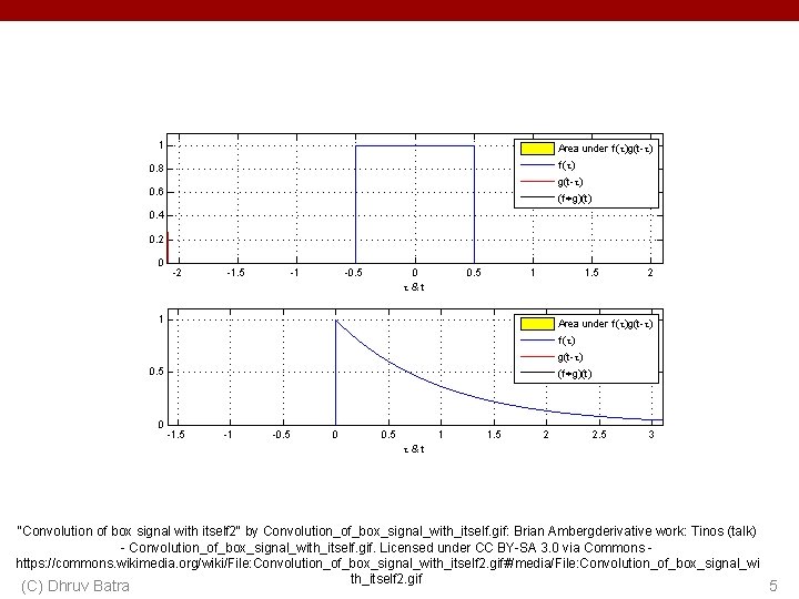
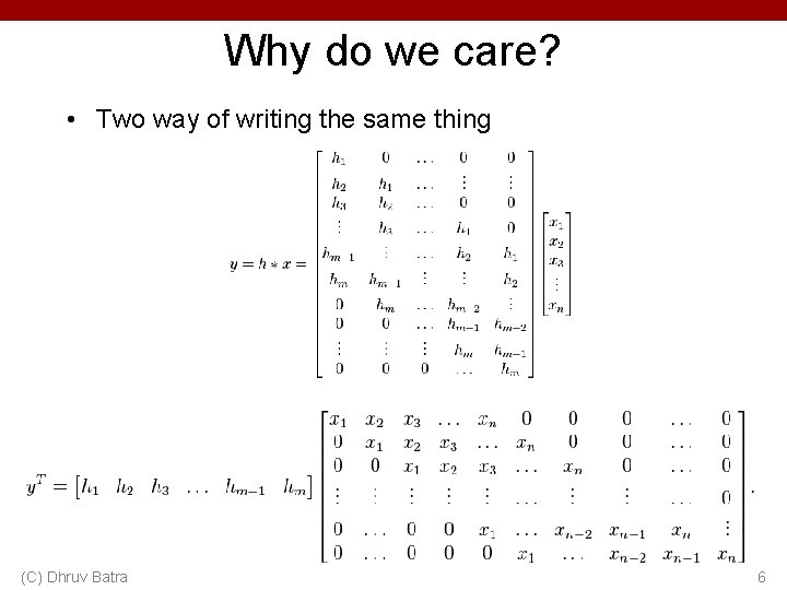
Why do we care? • (Discrete) Convolution = Matrix Multiplication – with Toeplitz Matrices (C) Dhruv Batra 4

"Convolution of box signal with itself 2" by Convolution_of_box_signal_with_itself. gif: Brian Ambergderivative work: Tinos (talk) - Convolution_of_box_signal_with_itself. gif. Licensed under CC BY-SA 3. 0 via Commons https: //commons. wikimedia. org/wiki/File: Convolution_of_box_signal_with_itself 2. gif#/media/File: Convolution_of_box_signal_wi th_itself 2. gif (C) Dhruv Batra 5

Why do we care? • Two way of writing the same thing (C) Dhruv Batra 6

Plan for Today • Toeplitz Matrix • 1 x 1 Convolution – AKA How to run a Conv. Net on arbitrary sized images (C) Dhruv Batra 7

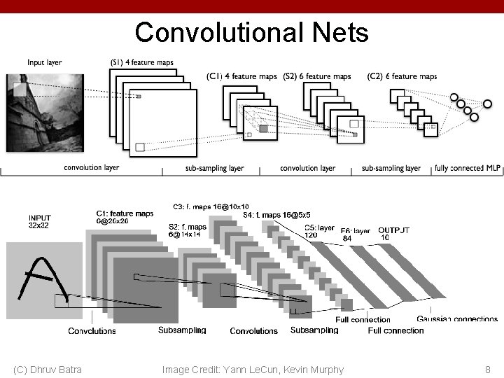
Convolutional Nets a (C) Dhruv Batra Image Credit: Yann Le. Cun, Kevin Murphy 8

Classical View (C) Dhruv Batra Figure Credit: [Long, Shelhamer, Darrell CVPR 15] 9

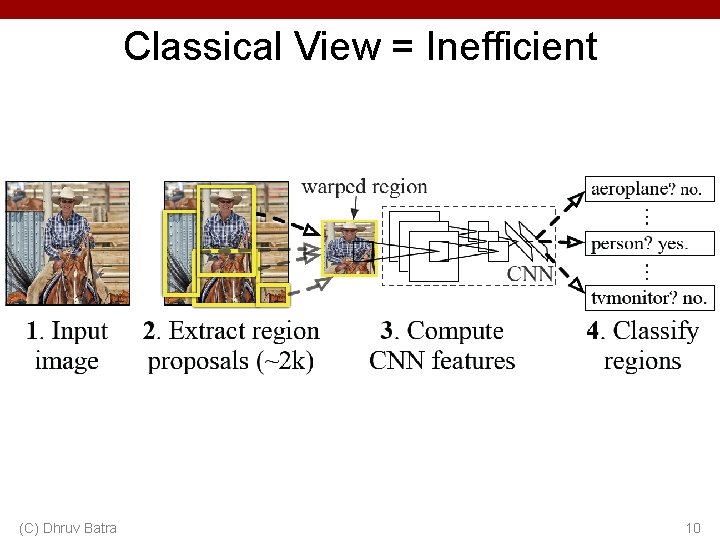
Classical View = Inefficient (C) Dhruv Batra 10

Classical View (C) Dhruv Batra Figure Credit: [Long, Shelhamer, Darrell CVPR 15] 11

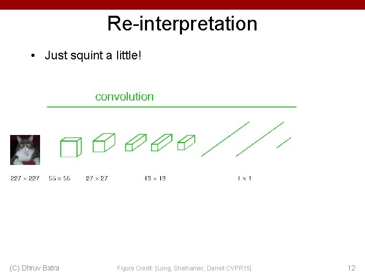
Re-interpretation • Just squint a little! (C) Dhruv Batra Figure Credit: [Long, Shelhamer, Darrell CVPR 15] 12

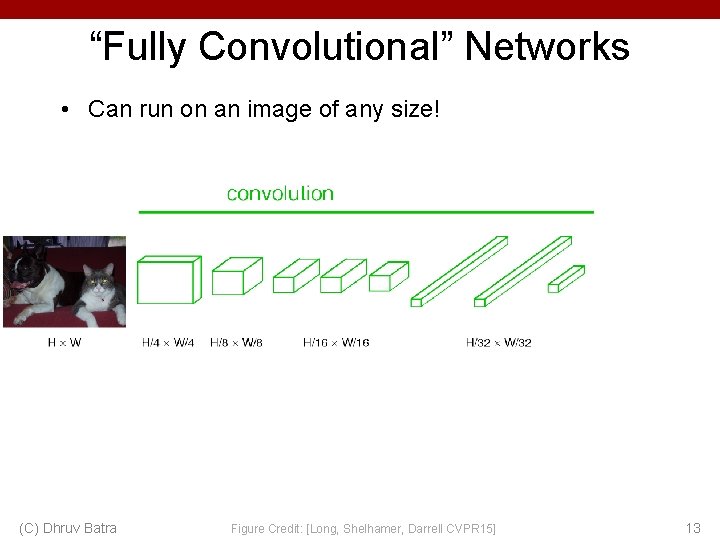
“Fully Convolutional” Networks • Can run on an image of any size! (C) Dhruv Batra Figure Credit: [Long, Shelhamer, Darrell CVPR 15] 13

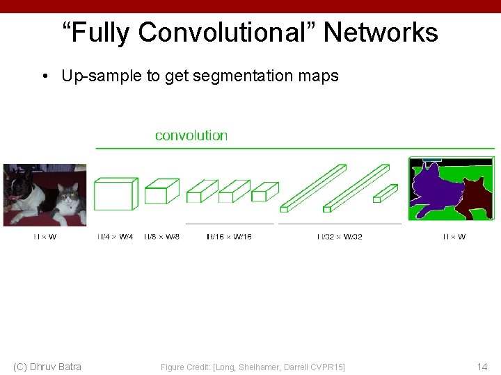
“Fully Convolutional” Networks • Up-sample to get segmentation maps (C) Dhruv Batra Figure Credit: [Long, Shelhamer, Darrell CVPR 15] 14

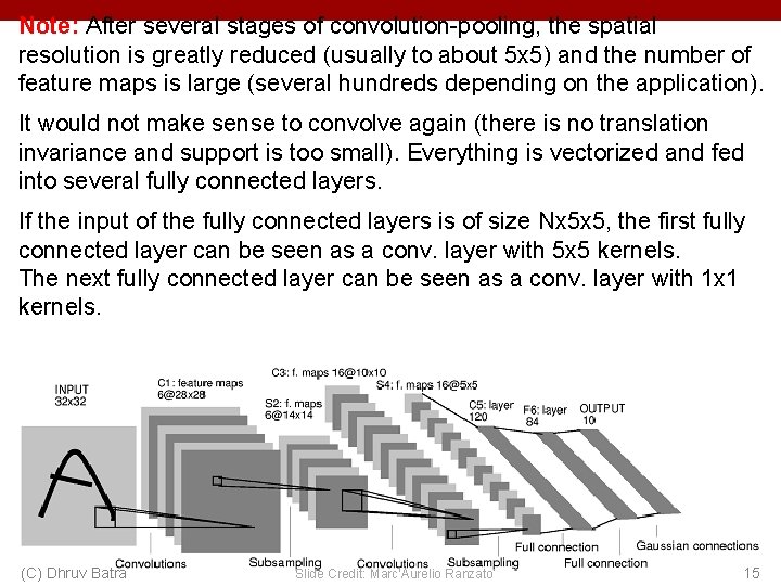
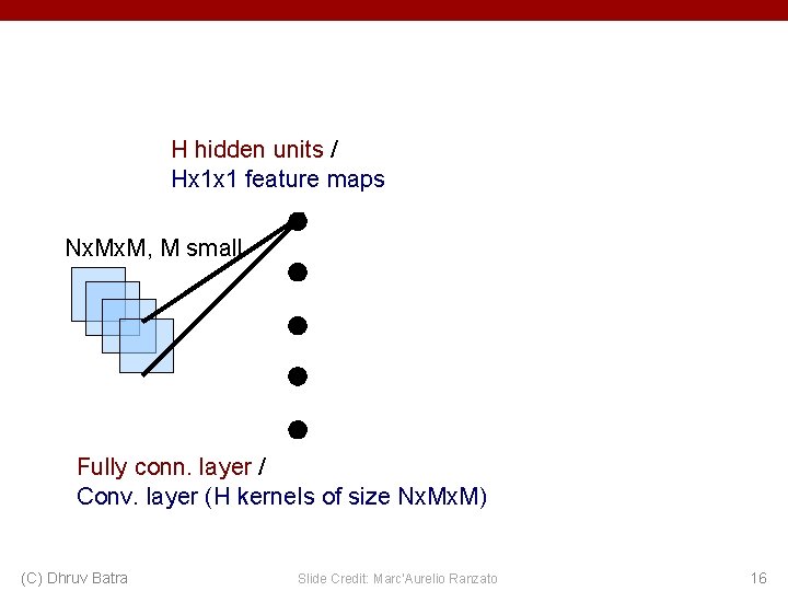
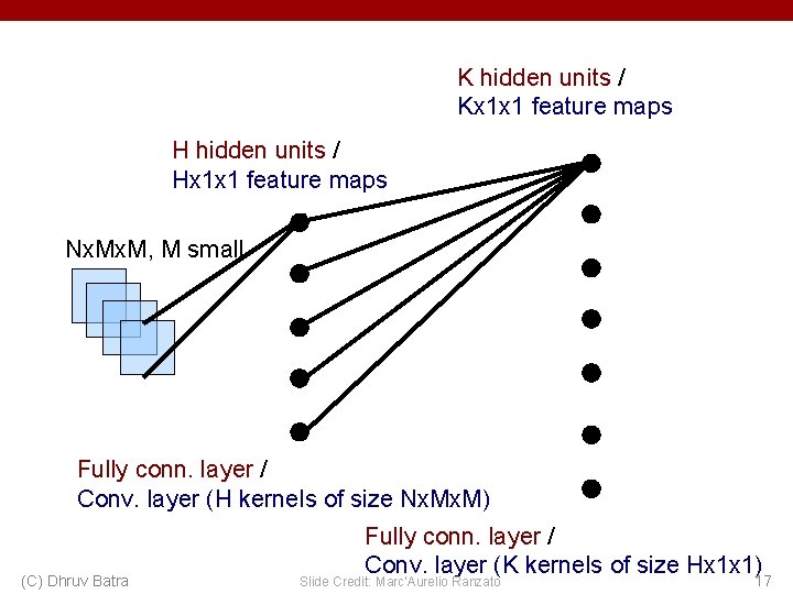
Note: After several stages of convolution-pooling, the spatial resolution is greatly reduced (usually to about 5 x 5) and the number of feature maps is large (several hundreds depending on the application). It would not make sense to convolve again (there is no translation invariance and support is too small). Everything is vectorized and fed into several fully connected layers. If the input of the fully connected layers is of size Nx 5 x 5, the first fully connected layer can be seen as a conv. layer with 5 x 5 kernels. The next fully connected layer can be seen as a conv. layer with 1 x 1 kernels. (C) Dhruv Batra Slide Credit: Marc'Aurelio Ranzato 15

H hidden units / Hx 1 x 1 feature maps Nx. M, M small Fully conn. layer / Conv. layer (H kernels of size Nx. M) (C) Dhruv Batra Slide Credit: Marc'Aurelio Ranzato 16

K hidden units / Kx 1 x 1 feature maps H hidden units / Hx 1 x 1 feature maps Nx. M, M small Fully conn. layer / Conv. layer (H kernels of size Nx. M) (C) Dhruv Batra Fully conn. layer / Conv. layer (K kernels of size Hx 1 x 1) Slide Credit: Marc'Aurelio Ranzato 17

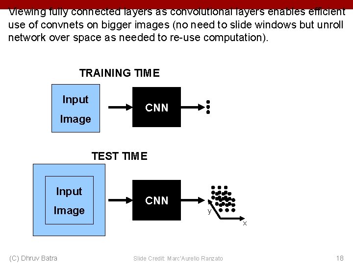
Viewing fully connected layers as convolutional layers enables efficient use of convnets on bigger images (no need to slide windows but unroll network over space as needed to re-use computation). TRAINING TIME Input Image CNN TEST TIME Input Image CNN y x (C) Dhruv Batra Slide Credit: Marc'Aurelio Ranzato 18

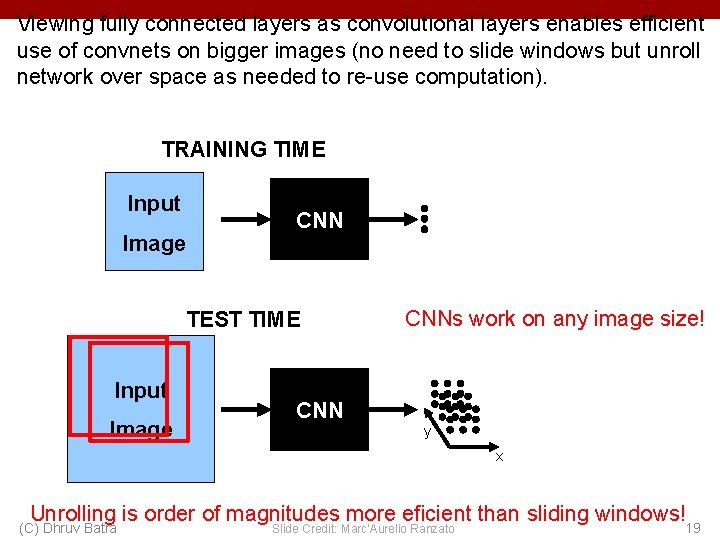
Viewing fully connected layers as convolutional layers enables efficient use of convnets on bigger images (no need to slide windows but unroll network over space as needed to re-use computation). TRAINING TIME Input Image CNN TEST TIME Input Image CNNs work on any image size! y x Unrolling is order of magnitudes more eficient than sliding windows! (C) Dhruv Batra Slide Credit: Marc'Aurelio Ranzato 19

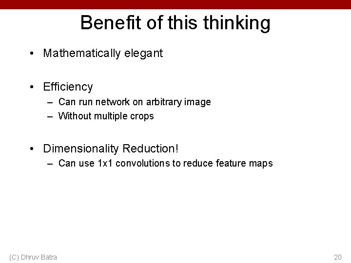
Benefit of this thinking • Mathematically elegant • Efficiency – Can run network on arbitrary image – Without multiple crops • Dimensionality Reduction! – Can use 1 x 1 convolutions to reduce feature maps (C) Dhruv Batra 20