DifferenceinDifference A Versatile Method for Quasi Experimental Evaluation

Difference-in-Difference: A Versatile Method for Quasi. Experimental Evaluation Roderick A. Rose, Ph. D Assistant Professor University of Maryland, Baltimore Christopher J. Wretman, Ph. D Senior Data Analyst University of North Carolina at Chapel Hill John A. Cosgrove, MSW Doctoral Candidate University of Maryland, Baltimore

Research for Social Change

Making Inferences About Change Social welfare research tests programs promoting social change. These interventions should be evidence-based, which requires scientific evidence that they work. “Scientific” implies a high standard that shows the intervention causes a change in a process or outcome. The “gold” standard is the randomized control trial

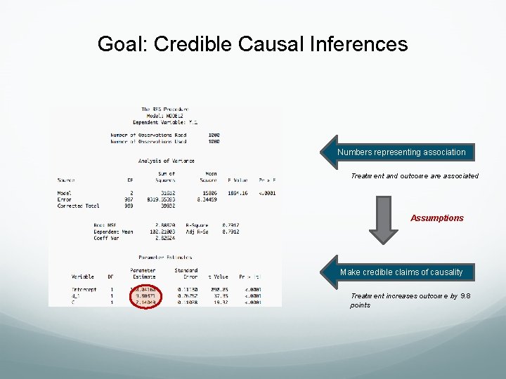
Goal: Credible Causal Inferences Numbers representing association Treatment and outcome are associated Assumptions Make credible claims of causality Treatment increases outcome by 9. 8 points

Randomized Control Trials A methodological approach: Measure differences in change across comparable groups to establish causal effects. A philosophical orientation: Comparable groups are best created via randomization. If randomization creates truly comparable groups, then the causal effects in our sample are equal to the true (but unknown) population treatment effect.

But we can’t always feasibly randomize! And gosh golly gee whillickers. . . sometimes we don’t even want to!

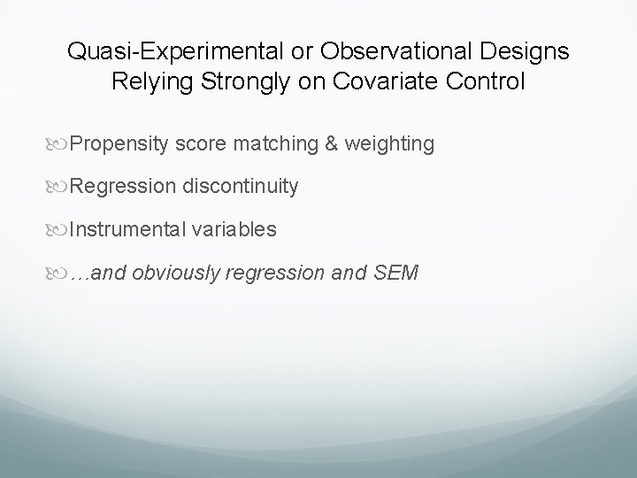
Quasi-Experimental or Observational Designs Relying Strongly on Covariate Control Propensity score matching & weighting Regression discontinuity Instrumental variables …and obviously regression and SEM

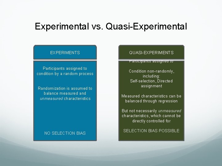
Experimental vs. Quasi-Experimental EXPERIMENTS QUASI-EXPERIMENTS Participants assigned to condition by a random process Randomization is assumed to balance measured and unmeasured characteristics Condition non-randomly, including: Self-selection, Directed assignment Measured characteristics can be balanced through regression But not necessarily unmeasured characteristics, which cannot be directly controlled for NO SELECTION BIAS POSSIBLE

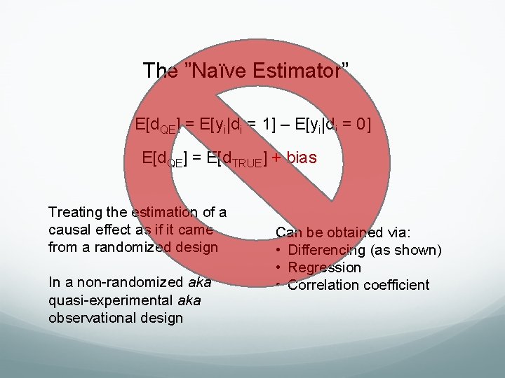
The ”Naïve Estimator” E[d. QE] = E[yi|di = 1] – E[yi|di = 0] E[d. QE] = E[d. TRUE] + bias Treating the estimation of a causal effect as if it came from a randomized design In a non-randomized aka quasi-experimental aka observational design Can be obtained via: • Differencing (as shown) • Regression • Correlation coefficient

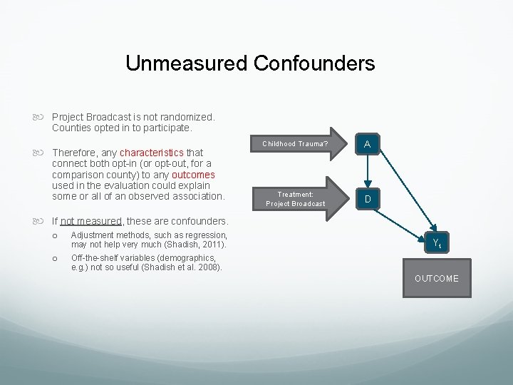
Unmeasured Confounders Project Broadcast is not randomized. Counties opted in to participate. Therefore, any characteristics that connect both opt-in (or opt-out, for a comparison county) to any outcomes used in the evaluation could explain some or all of an observed association. Childhood Trauma? A Treatment: Project Broadcast D If not measured, these are confounders. o Adjustment methods, such as regression, may not help very much (Shadish, 2011). o Off-the-shelf variables (demographics, e. g. ) not so useful (Shadish et al. 2008). Yt OUTCOME

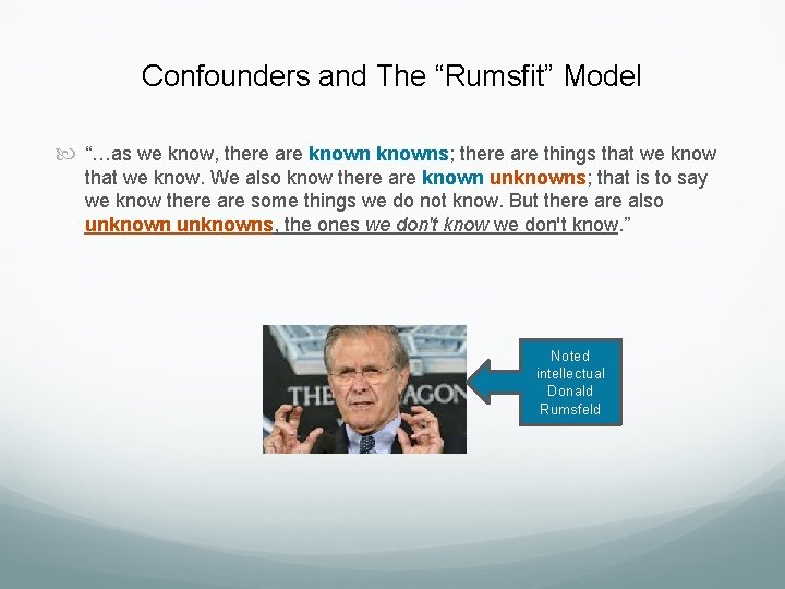
Confounders and The “Rumsfit” Model “…as we know, there are knowns; there are things that we know. We also know there are known unknowns; that is to say we know there are some things we do not know. But there also unknowns, the ones we don't know. ” Noted intellectual Donald Rumsfeld

The point of all this silliness is… We have blind spots that make it difficult to make certain claims. Wouldn’t it be nice to have a method that allows us to circumnavigate around the confounders problem, i. e. , allow us to adjust for the confounders without having the confounders? There a few of these, including DD.

DD: The Basic Framework

Difference-in-Difference (DD) A promising QE method that has received attention in econometric program evaluation. Useful when both pretest and posttest measures of the outcome are obtained. It is a very flexible method, with the potential to handle multiple (j > 2) treatment groups and multiple (t > 2) waves as well as simple 2 -group, 2 -period designs. It works in both panel/longitudinal and in serial cross-section designs. In the 2 -period panel setting, it is equivalent to the change score method.

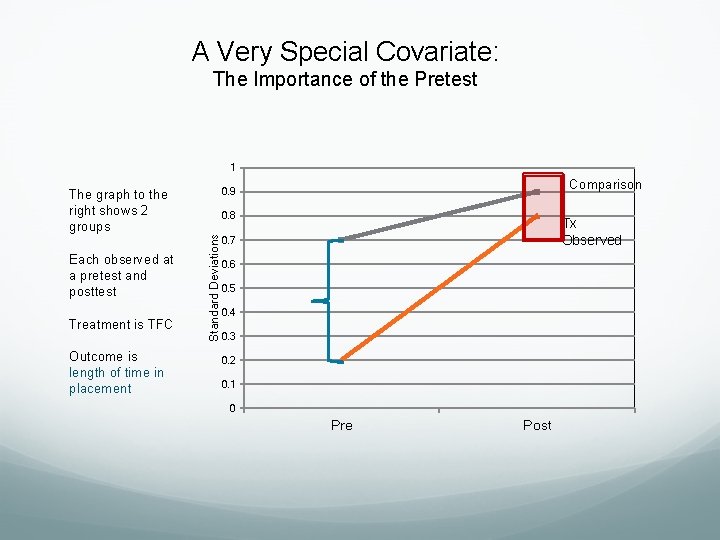
A Very Special Covariate: The Importance of the Pretest 1 Each observed at a pretest and posttest Treatment is TFC Outcome is length of time in placement Comparison 0. 9 0. 8 Standard Deviations The graph to the right shows 2 groups Tx Observed 0. 7 0. 6 0. 5 0. 4 0. 3 0. 2 0. 1 0 Pre Post

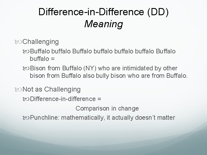
Difference-in-Difference (DD) Meaning Challenging Buffalo buffalo Buffalo buffalo = Bison from Buffalo (NY) who are intimidated by other bison from Buffalo also bully bison who are from Buffalo. Not as Challenging Difference-in-difference = Comparison in change Punchline: mathematically, it actually doesn’t matter

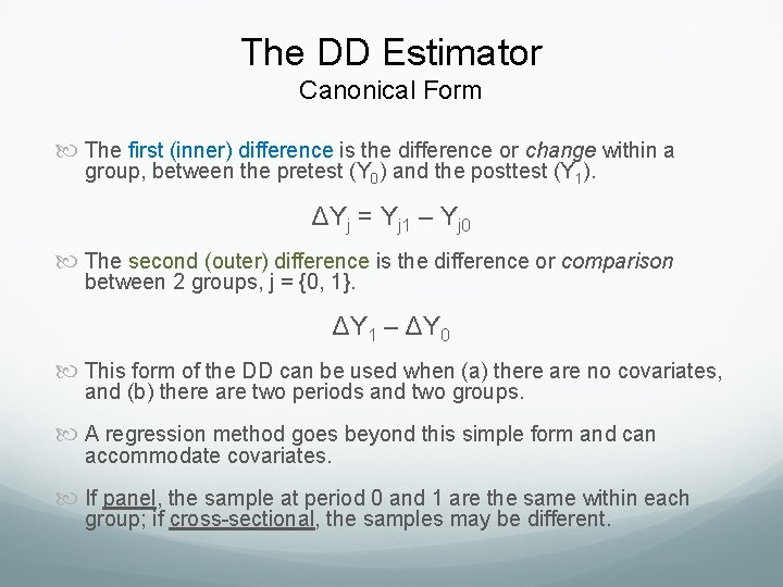
The DD Estimator Canonical Form The first (inner) difference is the difference or change within a group, between the pretest (Y 0) and the posttest (Y 1). ΔYj = Yj 1 – Yj 0 The second (outer) difference is the difference or comparison between 2 groups, j = {0, 1}. ΔY 1 – ΔY 0 This form of the DD can be used when (a) there are no covariates, and (b) there are two periods and two groups. A regression method goes beyond this simple form and can accommodate covariates. If panel, the sample at period 0 and 1 are the same within each group; if cross-sectional, the samples may be different.

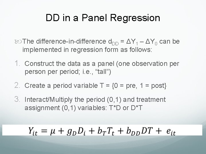
DD in a Panel Regression The difference-in-difference d. DD = ΔY 1 – ΔY 0 can be implemented in regression form as follows: 1. Construct the data as a panel (one observation person period; i. e. , “tall”) 2. Create a period variable T = {0 = pre, 1 = post} 3. Interact/Multiply the period (0, 1) and treatment assignment (0, 1) variables: T*D or D*T

DD Practicalities Example: 2 Period, 2 Group Design

Software DD can easily be defined analyzed in all major statistical software packages: R, SAS, SPSS, Stata, etc. A major appeal of DD is its analytic simplicity and ease of use. As always. . . procedures, options, output, frustrations, etc. will vary based on choice. For this workshop, we will present syntax and outputs using Stata. . .

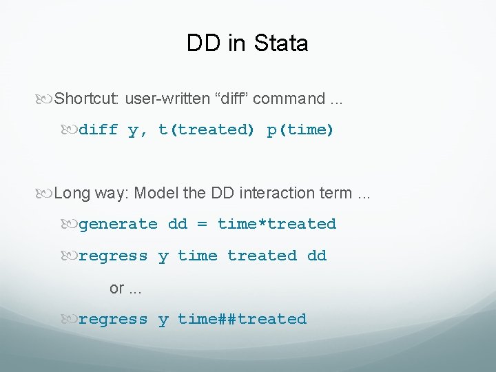
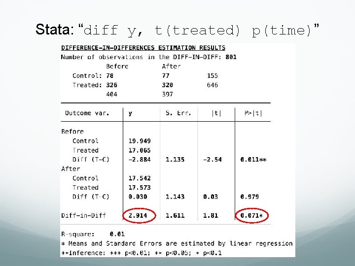
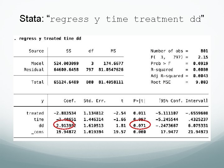
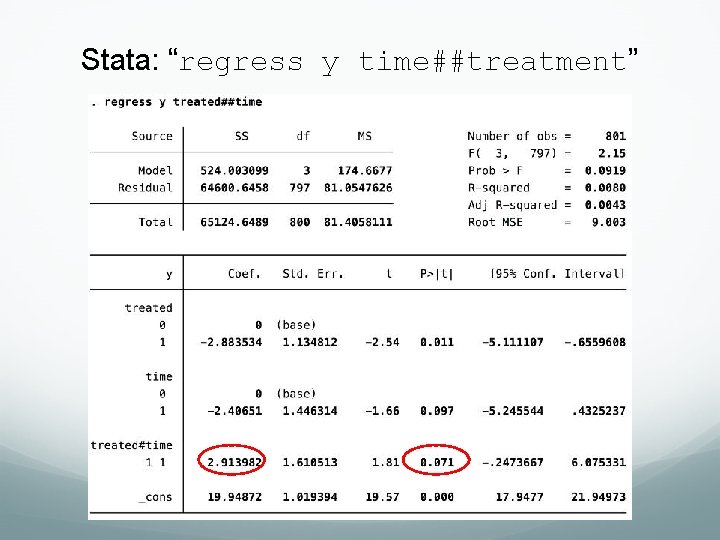
DD in Stata Shortcut: user-written “diff” command. . . diff y, t(treated) p(time) Long way: Model the DD interaction term. . . generate dd = time*treated regress y time treated dd or. . . regress y time##treated

Hypothetical Let us imagine we have randomized 810 adults with severe and persistent mental illness in two states into receiving either a weekly group-based employment intervention (1; New Jersey; N=662). . . or a weekly informational mailer (0; Pennsylvania; n=158). We measure their full time employment at baseline (0) and then after 5 months (1) to see if the intervention increased the employment of intervention participants relative to control.

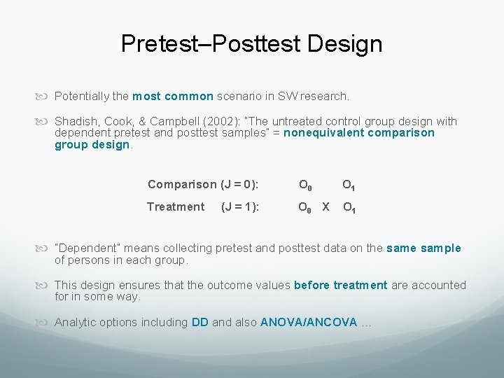
Pretest–Posttest Design Potentially the most common scenario in SW research. Shadish, Cook, & Campbell (2002): “The untreated control group design with dependent pretest and posttest samples” = nonequivalent comparison group design. Comparison (J = 0): O 0 O 1 Treatment O 0 X O 1 (J = 1): “Dependent” means collecting pretest and posttest data on the sample of persons in each group. This design ensures that the outcome values before treatment are accounted for in some way. Analytic options including DD and also ANOVA/ANCOVA. . .

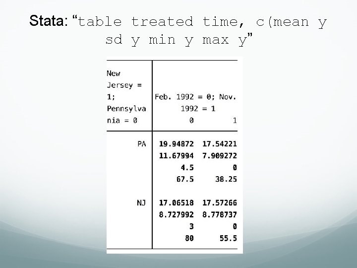
Stata: “table treated time, c(mean y sd y min y max y”

Stata: “diff y, t(treated) p(time)”

Stata: “regress y time treatment dd”

Stata: “regress y time##treatment”

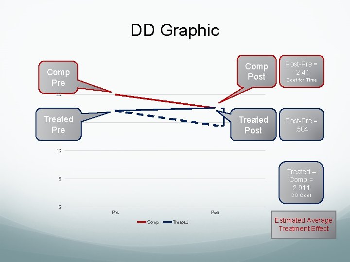
DD Graphic Comp Pre Comp Post-Pre = -2. 41 2. 914 Treated Post-Pre =. 504 Coef for Time 20 Treated 15 Pre 10 Treated – Comp = 2. 914 5 DD Coef 0 Pre Post Comp Treated Estimated Average Treatment Effect

Interpretation: “Results using a difference-in-differences analysis demonstrated an approaching significant (p=. 071) treatment effect whereby adults in the treatment group demonstrated an increase in full time employment relative to the control group. ”

How Do We Choose? Between DD and a Pre/Post ANOVA The relevant factor is whether treatment groups regress to a mean that is common to both groups: Yes: Pre/Post No: DD (Parallel Trends Assumption) With only 2 waves (periods) we cannot establish which is most likely true; instead we base our decision on design, e. g. : Yes: members are from a single population No: members are from different populations, such as different schools or counties

Next: A Better Design It is a general recommendation (not unique to DD) that we use multi-wave (repeated measures) designs Such designs can allow us to establish pretreatment change This would allow us to improve upon our educated guess about regression to a common mean In some cases we can even test the pre-treatment trend to see if the groups are moving towards each other

Longitudinal DD DD with Multiple Waves as a Panel Multilevel Model

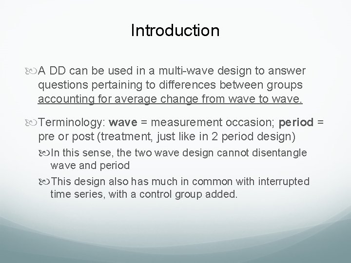
Introduction A DD can be used in a multi-wave design to answer questions pertaining to differences between groups accounting for average change from wave to wave. Terminology: wave = measurement occasion; period = pre or post (treatment, just like in 2 period design) In this sense, the two wave design cannot disentangle wave and period This design also has much in common with interrupted time series, with a control group added.

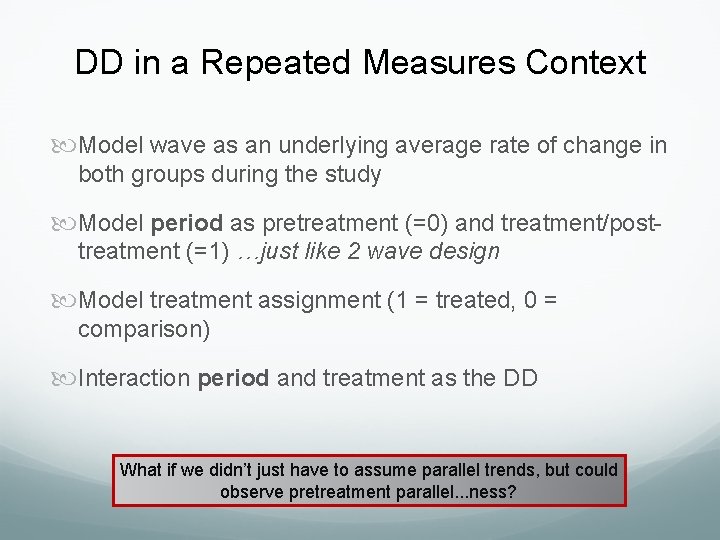
DD in a Repeated Measures Context Model wave as an underlying average rate of change in both groups during the study Model period as pretreatment (=0) and treatment/posttreatment (=1) …just like 2 wave design Model treatment assignment (1 = treated, 0 = comparison) Interaction period and treatment as the DD What if we didn’t just have to assume parallel trends, but could observe pretreatment parallel. . . ness?

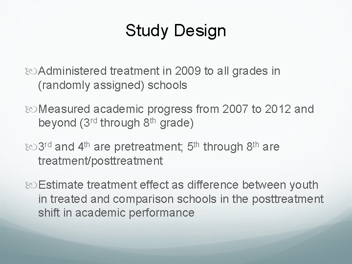
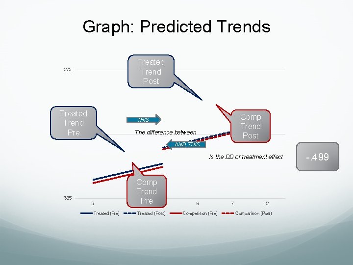
Study Design Administered treatment in 2009 to all grades in (randomly assigned) schools Measured academic progress from 2007 to 2012 and beyond (3 rd through 8 th grade) 3 rd and 4 th are pretreatment; 5 th through 8 th are treatment/posttreatment Estimate treatment effect as difference between youth in treated and comparison schools in the posttreatment shift in academic performance

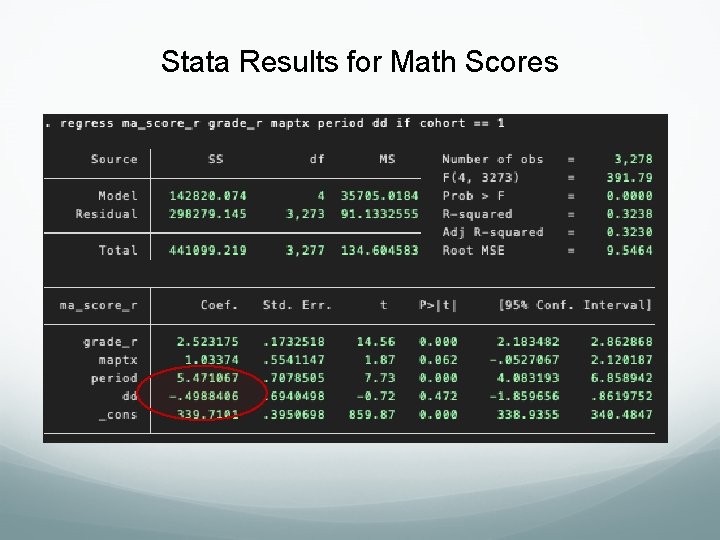
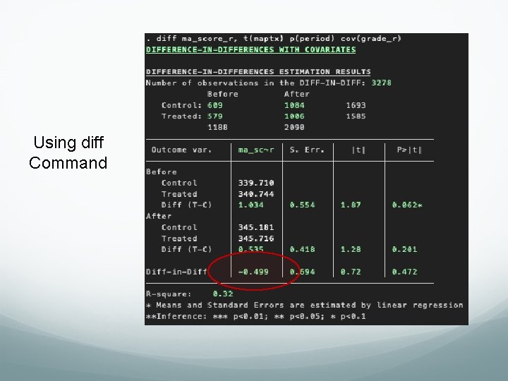
Stata Results for Math Scores

Using diff Command

Graph: Predicted Trends Treated Trend Post 375 Treated Trend Pre 355 Comp Trend Post THIS The difference between AND THIS Is the DD or treatment effect 335 3 Treated (Pre) 4 Comp Trend Pre 5 Treated (Post) 6 Comparison (Pre) 7 8 Comparison (Post) -. 499

Summary DD can accommodate multiwave data This is a repeated measures model with a shift beginning in the wave that the treatment starts The shift is different for the comparison (period marginal effect) and treatment (period marginal plus DD) This design is equivalently an interrupted time series design with comparison group Allows us to weaken our assumption of parallel trends or even investigate if it is plausible.

Simulation Test Does DD Estimate the True Treatment Effect?

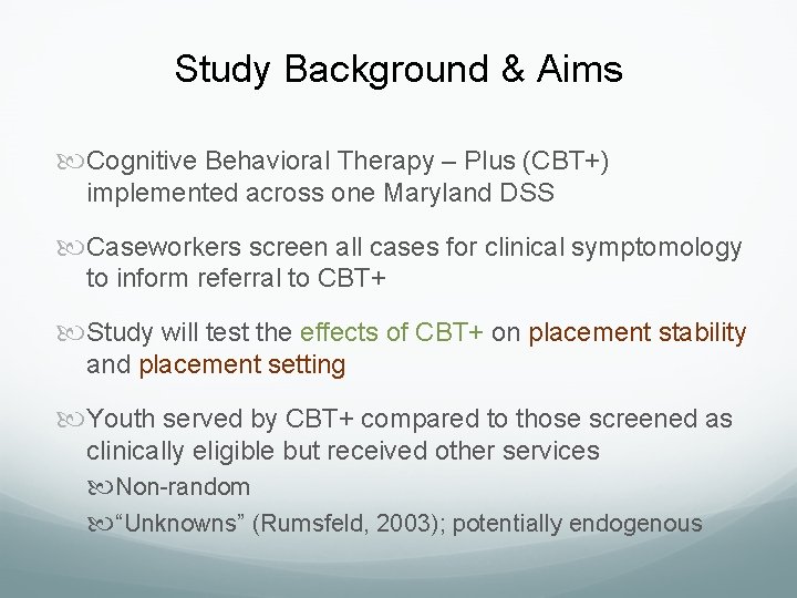
Study Background & Aims Cognitive Behavioral Therapy – Plus (CBT+) implemented across one Maryland DSS Caseworkers screen all cases for clinical symptomology to inform referral to CBT+ Study will test the effects of CBT+ on placement stability and placement setting Youth served by CBT+ compared to those screened as clinically eligible but received other services Non-random “Unknowns” (Rumsfeld, 2003); potentially endogenous

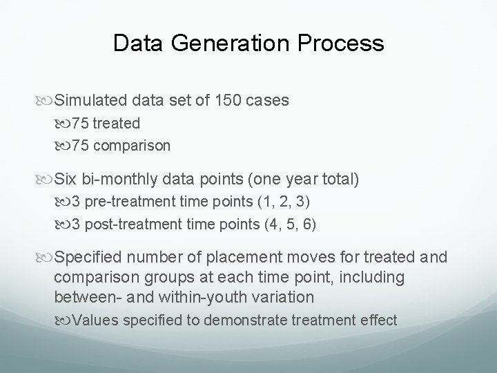
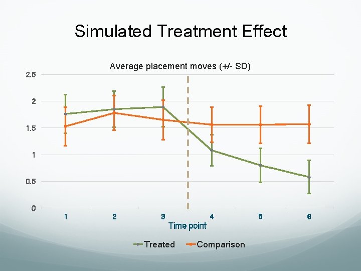
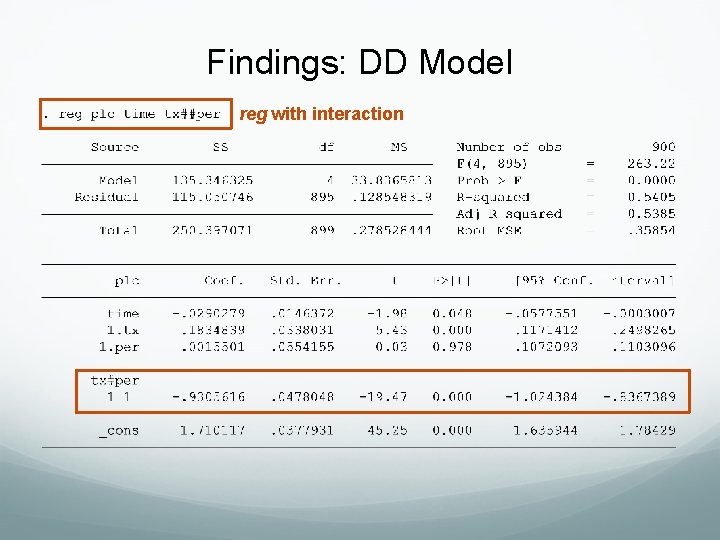
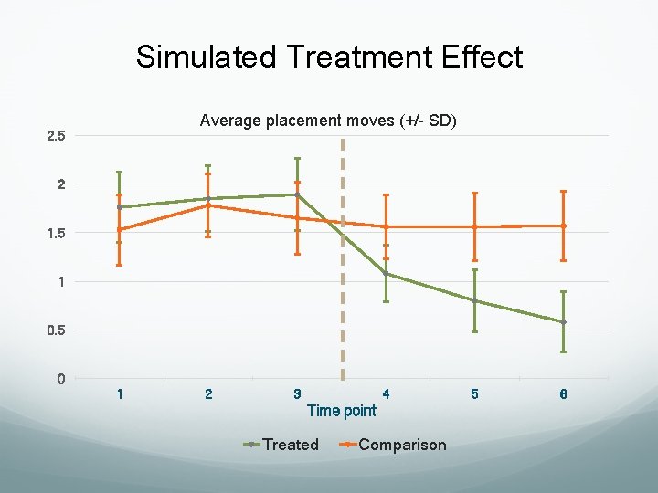
Data Generation Process Simulated data set of 150 cases 75 treated 75 comparison Six bi-monthly data points (one year total) 3 pre-treatment time points (1, 2, 3) 3 post-treatment time points (4, 5, 6) Specified number of placement moves for treated and comparison groups at each time point, including between- and within-youth variation Values specified to demonstrate treatment effect

Simulated Treatment Effect Average placement moves (+/- SD) 2. 5 2 1. 5 1 0. 5 0 1 2 3 4 Time point Treated Comparison 5 6

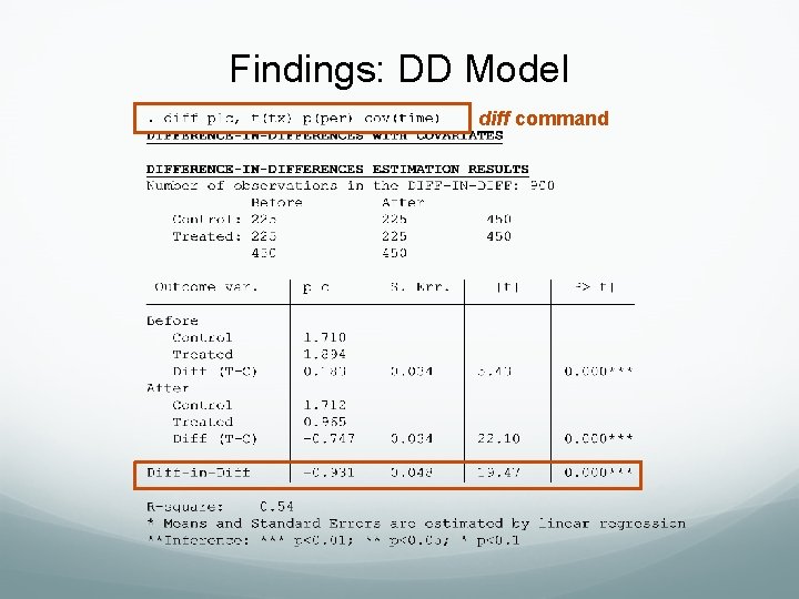
Findings: DD Model diff command

Findings: DD Model reg with interaction

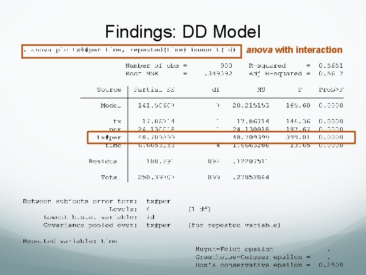
Findings: DD Model anova with interaction

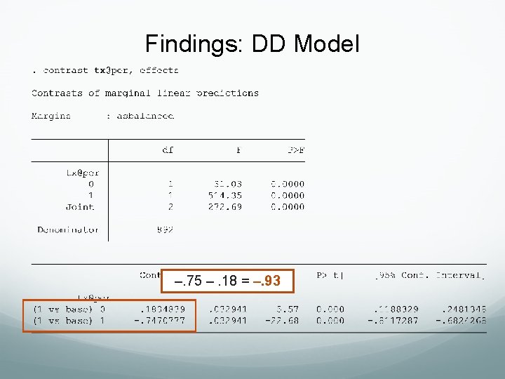
Findings: DD Model –. 75 –. 18 = –. 93

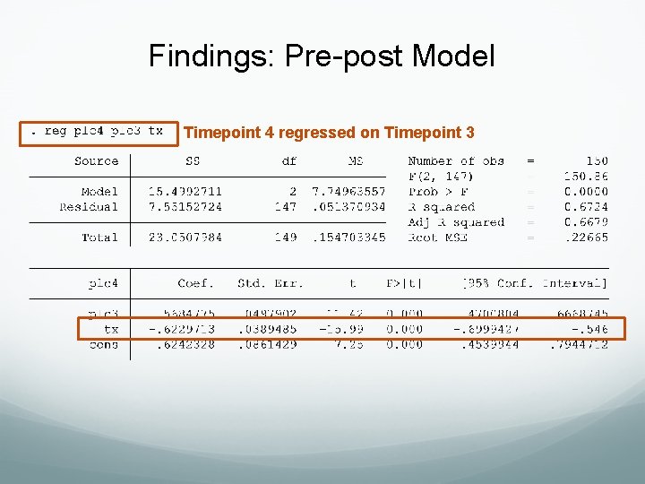
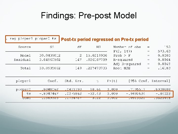
Findings: Pre-post Model Timepoint 4 regressed on Timepoint 3

Findings: Pre-post Model Post-tx period regressed on Pre-tx period

Simulated Treatment Effect Average placement moves (+/- SD) 2. 5 2 1. 5 1 0. 5 0 1 2 3 4 Time point Treated Comparison 5 6

Next Steps & Challenges Simulations show DD as a promising method for estimating CBT+ treatment effects Potential challenges with real-world evaluation data Distribution of placement change (positively skewed, over -dispersed) Parallel trends assumption not met Variation in placement time before and after treatment period (non-random)

Final Remarks

DD Limitations Inflates SEs. . . Can reduce power in comparison with other methods (e. g. , ANCOVA) Estimates are biased if there are pretreatment differences between groups …perhaps better to use pre/post design, or better yet, ensure repeated pretreatment measures and actually adjust for pretreatment differences in status and change

Further Insights into DD The DD can be extended to variations that not only account for a shift at the point of treatment, but a change in slope This would be a DDD (Buffalo buffalo…) The number of Ds indicating the order of the interaction The key assumption is the parallel trend Nonlinear models require certain accommodations

Literature Difference-in-difference Rose, R. A. & Bowen, N. K. (2019). Difference-in-differences as an alternative to pretest-posttest regression for social work intervention evaluation and research. Social Work Research 43(4), 247 -258. Schilling, S. , Shanahan, M. , Lanier, P. , Zolotor, A. , & Rose, R. A. (Online first. ) A quasi-experimental effectiveness study of Triple P on Child Maltreatment. Journal of Family Violence. Published online 22 Feb 2019. Causal Inference Rose, R. A. (2019). Frameworks for credible causal inference in observational studies of family violence. Journal of Family Violence 34(8), 690 -710. Rose, R. A. (2019). No credibility without plausibility: A response to Lewis and Lanier. Journal of Family Violence 34(8), 719 -722.

DD Literature Pischke, J-S. (2005). Empirical Methods in Applied Economics Lecture Notes. Available at http: //econ. lse. ac. uk/staff/spischke/ec 524/evaluation 3. pdf Barnighausen et al. (2017). Quasi-experimental design series— paper 7: assessing the assumptions. Journal of Clinical Epidemiology 89, 53 -66.