Designing Experiments Introduction 2 k factorial designs 2

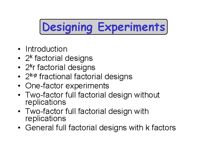
Designing Experiments • • • Introduction 2 k factorial designs 2 kr factorial designs 2 k-p fractional factorial designs One-factor experiments Two-factor full factorial design without replications • Two-factor full factorial design with replications • General full factorial designs with k factors

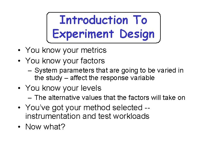
Introduction To Experiment Design • You know your metrics • You know your factors – System parameters that are going to be varied in the study – affect the response variable • You know your levels – The alternative values that the factors will take on • You’ve got your method selected -instrumentation and test workloads • Now what?

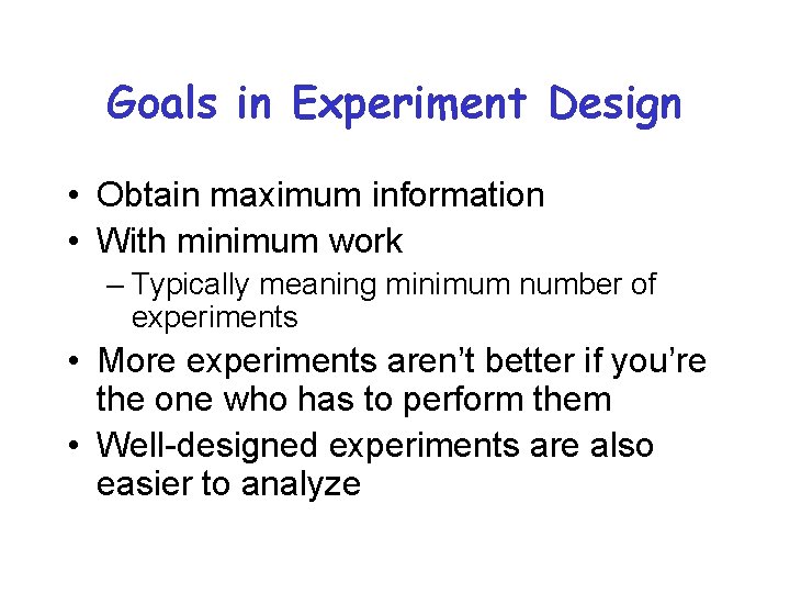
Goals in Experiment Design • Obtain maximum information • With minimum work – Typically meaning minimum number of experiments • More experiments aren’t better if you’re the one who has to perform them • Well-designed experiments are also easier to analyze

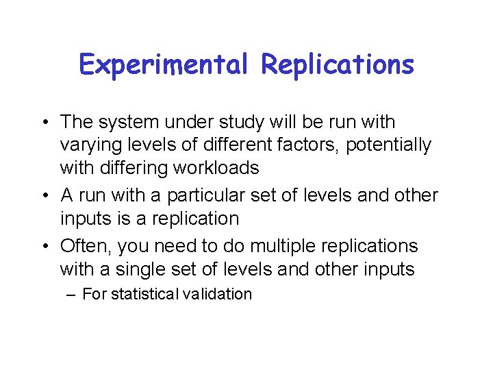
Experimental Replications • The system under study will be run with varying levels of different factors, potentially with differing workloads • A run with a particular set of levels and other inputs is a replication • Often, you need to do multiple replications with a single set of levels and other inputs – For statistical validation

Interacting Factors • Some factors have effects completely independent of each other – Doubling the factor’s level may halve the response, regardless of other factors • But the effects of some factors depends on the values of other factors – Interacting factors • Presence of interacting factors complicates experimental design

Basic Problem in Designing Experiments • You have chosen some number of factors • They may or may not interact • How can you design an experiment that captures the full range of the levels? – With minimum amount of work • Which combination or combinations of the levels of the factors do you measure?

Common Mistakes in Experimentation • • • Ignoring experimental error Uncontrolled parameters Not isolating effects of different factors One-factor-at-a-time experiment designs Interactions ignored Designs require too many experiments

Types of Experimental Designs • Simple designs • Full factorial design • Fractional factorial design

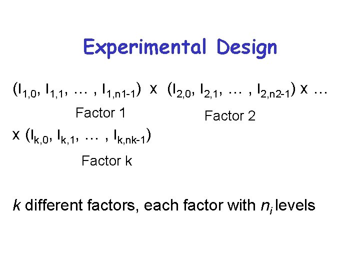
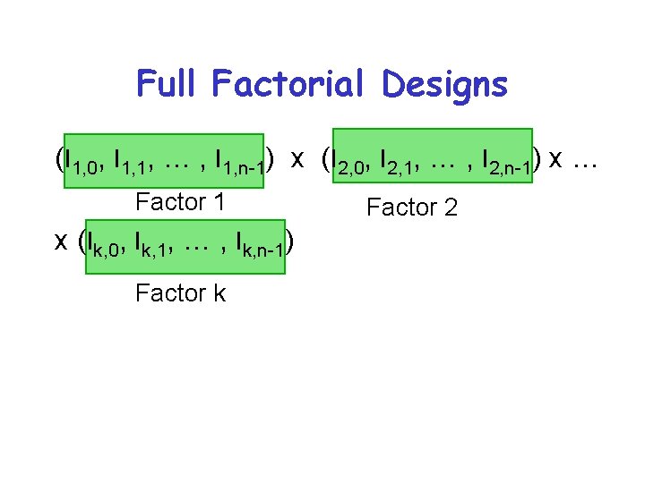
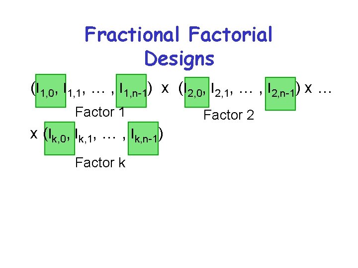
Experimental Design (l 1, 0, l 1, 1, … , l 1, n 1 -1) x (l 2, 0, l 2, 1, … , l 2, n 2 -1) x … Factor 1 Factor 2 x (lk, 0, lk, 1, … , lk, nk-1) Factor k k different factors, each factor with ni levels

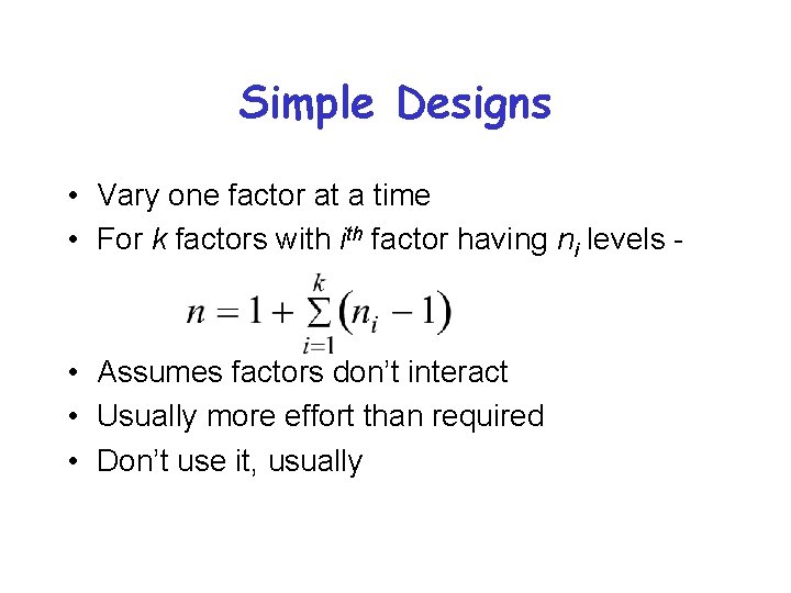
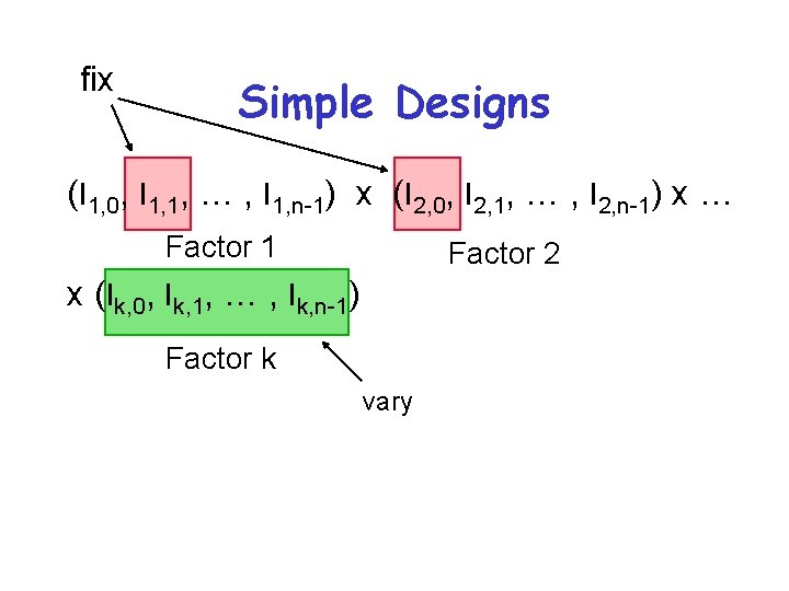
Simple Designs • Vary one factor at a time • For k factors with factor having ni levels - • Assumes factors don’t interact • Usually more effort than required • Don’t use it, usually

fix Simple Designs (l 1, 0, l 1, 1, … , l 1, n-1) x (l 2, 0, l 2, 1, … , l 2, n-1) x … Factor 1 Factor 2 x (lk, 0, lk, 1, … , lk, n-1) Factor k vary

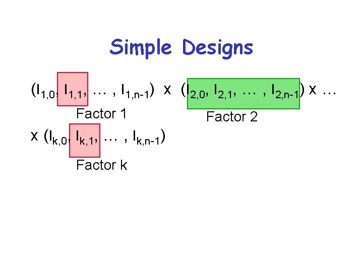
Simple Designs (l 1, 0, l 1, 1, … , l 1, n-1) x (l 2, 0, l 2, 1, … , l 2, n-1) x … Factor 1 x (lk, 0, lk, 1, … , lk, n-1) Factor k Factor 2

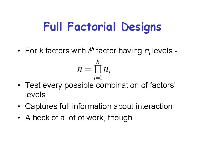
Full Factorial Designs • For k factors with factor having ni levels - • Test every possible combination of factors’ levels • Captures full information about interaction • A heck of a lot of work, though

Full Factorial Designs (l 1, 0, l 1, 1, … , l 1, n-1) x (l 2, 0, l 2, 1, … , l 2, n-1) x … Factor 1 x (lk, 0, lk, 1, … , lk, n-1) Factor k Factor 2

Reducing the Work in Full Factorial Designs • Reduce number of levels per factor – Generally a good choice – Especially if you know which factors are most important - use more levels for them • Reduce the number of factors – But don’t drop important ones • Use fractional factorial designs

Fractional Factorial Designs • Only measure some combination of the levels of the factors • Must design carefully to best capture any possible interactions • Less work, but more chance of inaccuracy • Especially useful if some factors are known not to interact

Fractional Factorial Designs (l 1, 0, l 1, 1, … , l 1, n-1) x (l 2, 0, l 2, 1, … , l 2, n-1) x … Factor 1 x (lk, 0, lk, 1, … , lk, n-1) Factor k Factor 2

2 k Factorial Designs • Used to determine the effect of k factors – Each with two alternatives or levels • Often used as a preliminary to a larger performance study – Each factor measured at its maximum and minimum level – Perhaps offering insight on importance and interaction of various factors

Unidirectional Effects • Effects that only increase as the level of a factor increases – Or visa versa • If this characteristic is known to apply, a 2 k factorial design at minimum and maximum levels is useful • Shows whether the factor has a significant effect

22 Factorial Designs • Two factors with two levels each • Simplest kind of factorial experiment design • Concepts developed here generalize • A form of regression can be easily used here • Simplest to show with an example

22 Factorial Design Example • The Time Warp Operating System • Designed to run discrete event simulations in parallel • Using an optimistic method • Goal is fastest possible completion of a given simulation • Usually quality is expressed in terms of speedup • Here, the simpler metric of runtime is used

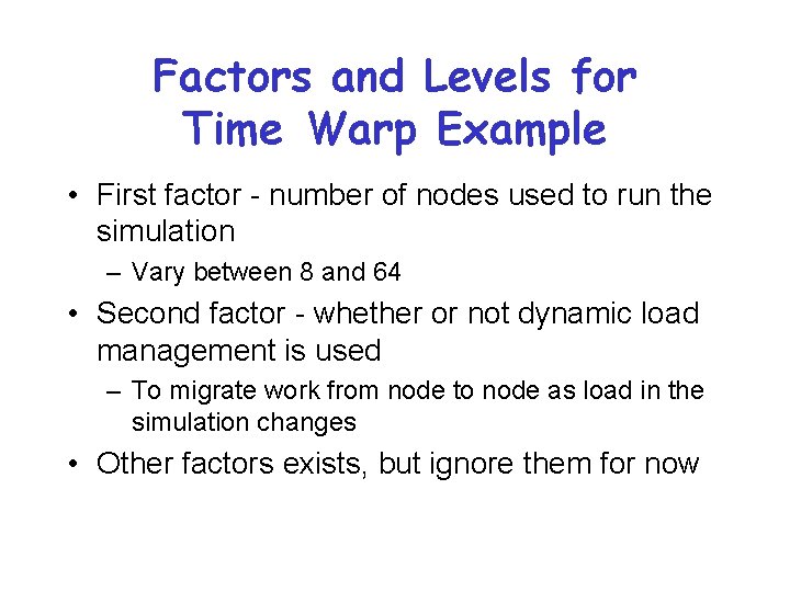
Factors and Levels for Time Warp Example • First factor - number of nodes used to run the simulation – Vary between 8 and 64 • Second factor - whether or not dynamic load management is used – To migrate work from node to node as load in the simulation changes • Other factors exists, but ignore them for now

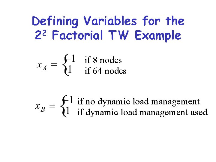
Defining Variables for the 22 Factorial TW Example if 8 nodes if 64 nodes if no dynamic load management if dynamic load management used

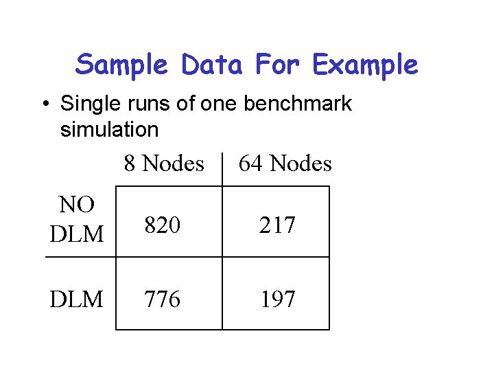
Sample Data For Example • Single runs of one benchmark simulation 8 Nodes 64 Nodes NO DLM 820 217 DLM 776 197

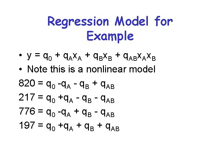
Regression Model for Example • y = q 0 + q. Ax. A + q. Bx. B + q. ABx. Ax. B • Note this is a nonlinear model 820 = q 0 -q. A - q. B + q. AB 217 = q 0 +q. A - q. B - q. AB 776 = q 0 -q. A + q. B - q. AB 197 = q 0 +q. A + q. B + q. AB

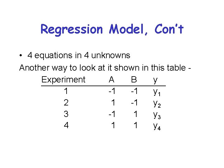
Regression Model, Con’t • 4 equations in 4 unknowns Another way to look at it shown in this table Experiment A B y 1 -1 -1 y 1 2 1 -1 y 2 3 -1 1 y 3 4 1 1 y 4

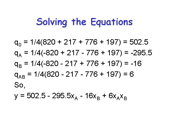
Solving the Equations q 0 = 1/4(820 + 217 + 776 + 197) = 502. 5 q. A = 1/4(-820 + 217 - 776 + 197) = -295. 5 q. B = 1/4(-820 - 217 + 776 + 197) = -16 q. AB = 1/4(820 - 217 - 776 + 197) = 6 So, y = 502. 5 - 295. 5 x. A - 16 x. B + 6 x. Ax. B

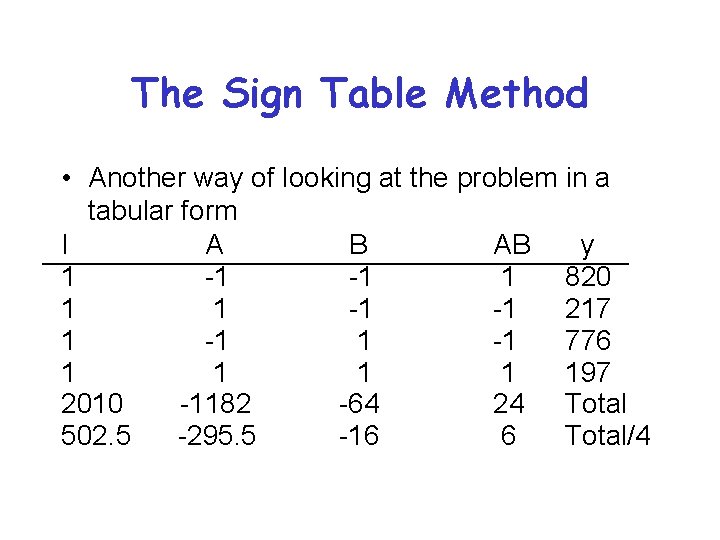
The Sign Table Method • Another way of looking at the problem in a tabular form I A B AB y 1 -1 -1 1 820 1 1 -1 -1 217 1 -1 776 1 1 197 2010 -1182 -64 24 Total 502. 5 -295. 5 -16 6 Total/4

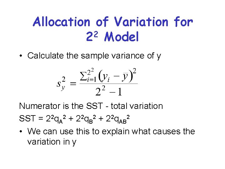
Allocation of Variation for 22 Model • Calculate the sample variance of y Numerator is the SST - total variation SST = 22 q. A 2 + 22 q. B 2 + 22 q. AB 2 • We can use this to explain what causes the variation in y

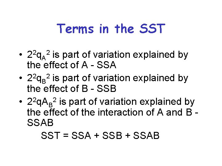
Terms in the SST • 22 q. A 2 is part of variation explained by the effect of A - SSA • 22 q. B 2 is part of variation explained by the effect of B - SSB • 22 q. AB 2 is part of variation explained by the effect of the interaction of A and B SSAB SST = SSA + SSB + SSAB

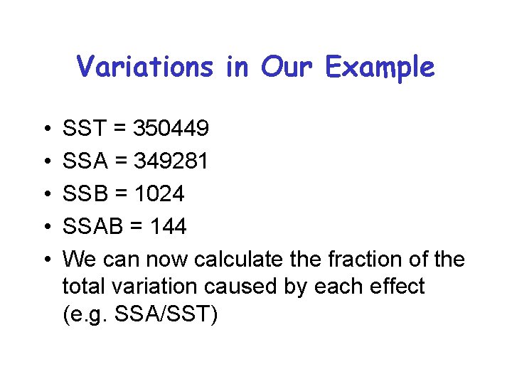
Variations in Our Example • • • SST = 350449 SSA = 349281 SSB = 1024 SSAB = 144 We can now calculate the fraction of the total variation caused by each effect (e. g. SSA/SST)

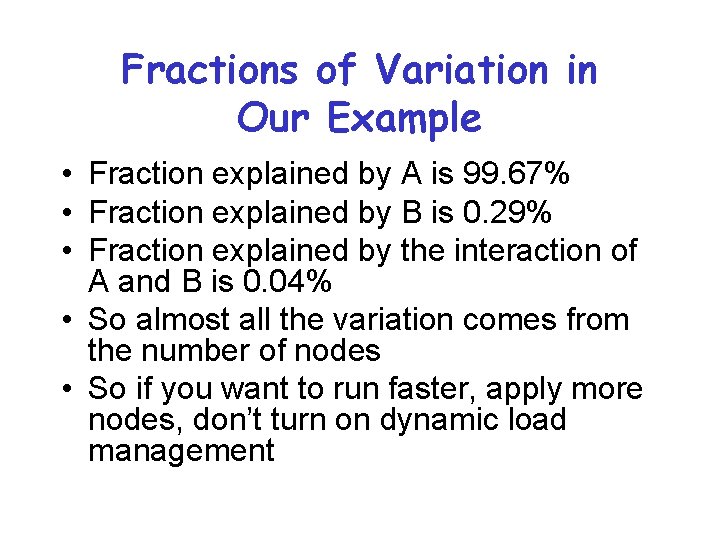
Fractions of Variation in Our Example • Fraction explained by A is 99. 67% • Fraction explained by B is 0. 29% • Fraction explained by the interaction of A and B is 0. 04% • So almost all the variation comes from the number of nodes • So if you want to run faster, apply more nodes, don’t turn on dynamic load management

General 2 k Factorial Designs • Used to explain the effects of k factors, each with two alternatives or levels • 22 factorial designs are a special case • Methods developed there extend to the more general case • But many more possible interactions between pairs (and trios, etc. ) of factors

2 k Factorial Designs With Replications • 2 k factorial designs do not allow for estimation of experimental error – No experiment is ever repeated • But usually experimental error is present – And often it’s important • Handle the issue by replicating experiments • But which to replicate, and how often?

2 kr Factorial Designs • Replicate each experiment r times • Allows quantification of experimental error • Again, easiest to first look at the case of only 2 factors

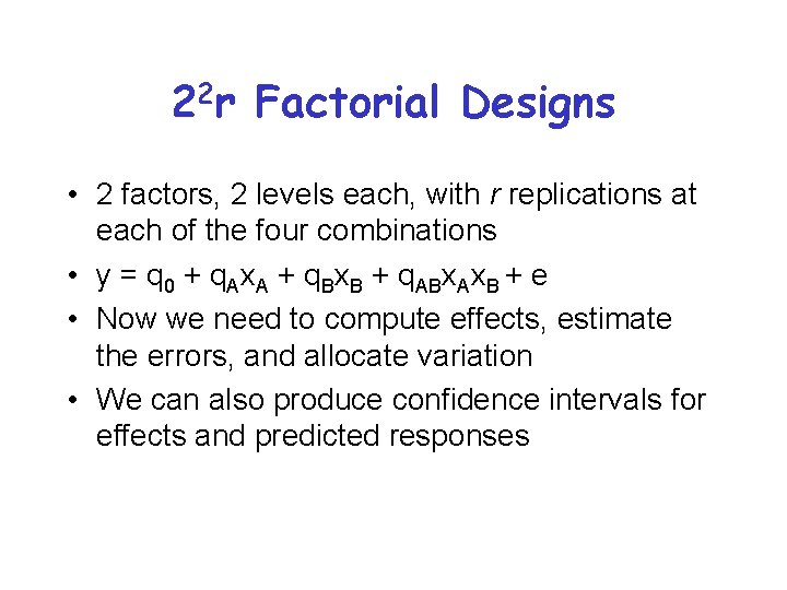
22 r Factorial Designs • 2 factors, 2 levels each, with r replications at each of the four combinations • y = q 0 + q. Ax. A + q. Bx. B + q. ABx. Ax. B + e • Now we need to compute effects, estimate the errors, and allocate variation • We can also produce confidence intervals for effects and predicted responses

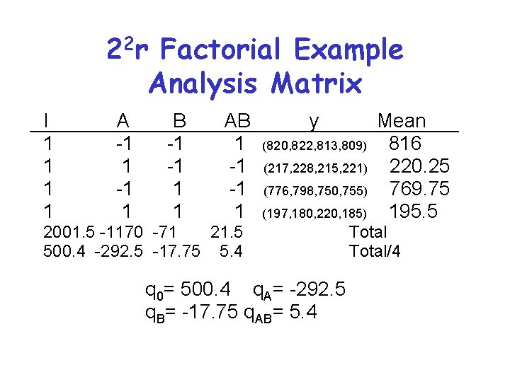
Computing Effects for 22 r Factorial Experiments • We can use the sign table, as before • But instead of single observations, regress off the mean of the r observations • Compute errors for each replication using similar tabular method • Similar methods used for allocation of variance and calculating confidence intervals

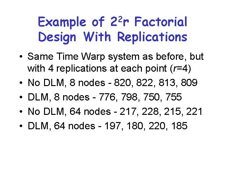
Example of 22 r Factorial Design With Replications • Same Time Warp system as before, but with 4 replications at each point (r=4) • No DLM, 8 nodes - 820, 822, 813, 809 • DLM, 8 nodes - 776, 798, 750, 755 • No DLM, 64 nodes - 217, 228, 215, 221 • DLM, 64 nodes - 197, 180, 220, 185

22 r Factorial Example Analysis Matrix I 1 1 A -1 1 B -1 -1 1 1 AB 1 -1 -1 1 y (820, 822, 813, 809) (217, 228, 215, 221) (776, 798, 750, 755) (197, 180, 220, 185) 2001. 5 -1170 -71 21. 5 500. 4 -292. 5 -17. 75 5. 4 q 0= 500. 4 q. A= -292. 5 q. B= -17. 75 q. AB= 5. 4 Mean 816 220. 25 769. 75 195. 5 Total/4

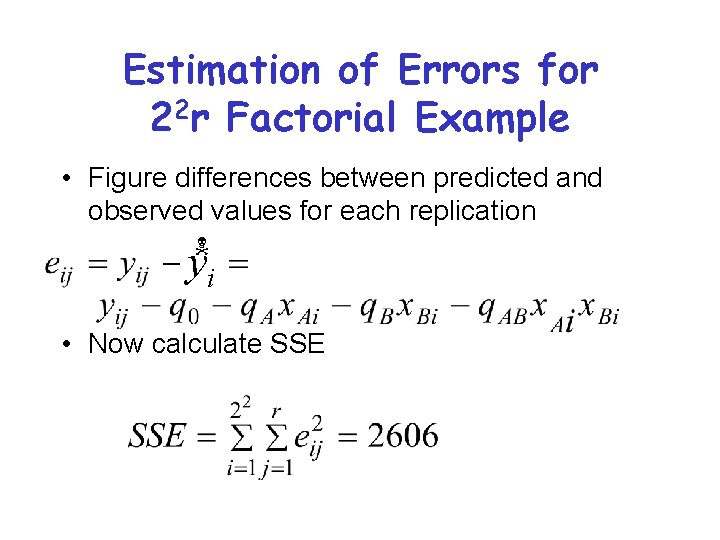
Estimation of Errors for 22 r Factorial Example • Figure differences between predicted and observed values for each replication N yi • Now calculate SSE

Allocating Variation • We can determine the percentage of variation due to each factor’s impact – Just like 2 k designs without replication • But we can also isolate the variation due to experimental errors • Methods are similar to other regression techniques for allocating variation

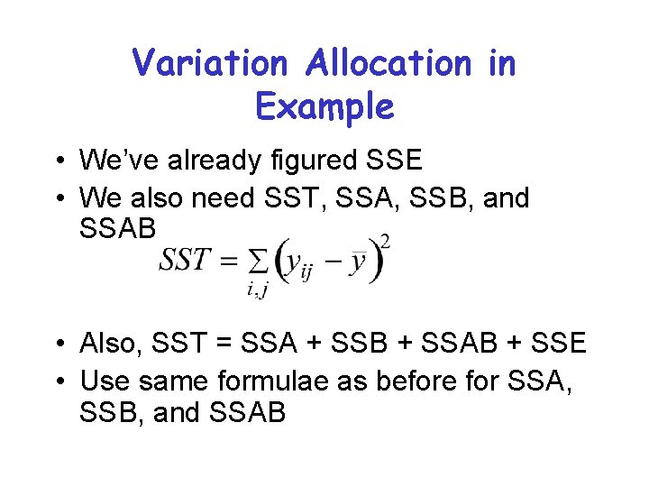
Variation Allocation in Example • We’ve already figured SSE • We also need SST, SSA, SSB, and SSAB • Also, SST = SSA + SSB + SSAB + SSE • Use same formulae as before for SSA, SSB, and SSAB

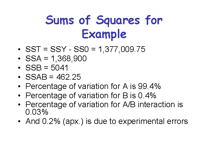
Sums of Squares for Example • • SST = SSY - SS 0 = 1, 377, 009. 75 SSA = 1, 368, 900 SSB = 5041 SSAB = 462. 25 Percentage of variation for A is 99. 4% Percentage of variation for B is 0. 4% Percentage of variation for A/B interaction is 0. 03% • And 0. 2% (apx. ) is due to experimental errors

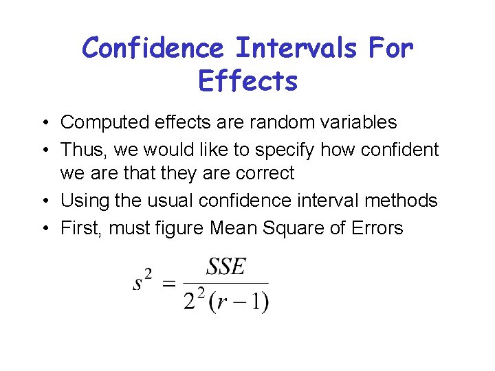
Confidence Intervals For Effects • Computed effects are random variables • Thus, we would like to specify how confident we are that they are correct • Using the usual confidence interval methods • First, must figure Mean Square of Errors

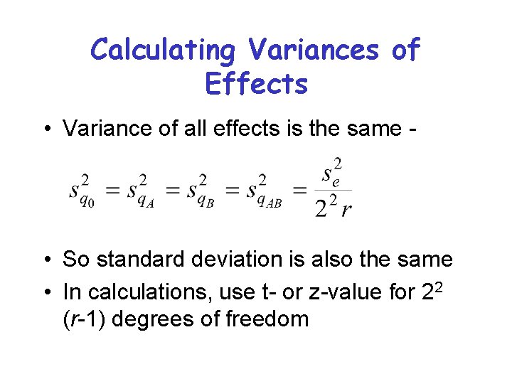
Calculating Variances of Effects • Variance of all effects is the same - • So standard deviation is also the same • In calculations, use t- or z-value for 22 (r-1) degrees of freedom

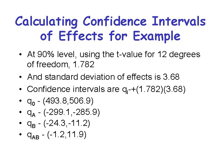
Calculating Confidence Intervals of Effects for Example • At 90% level, using the t-value for 12 degrees of freedom, 1. 782 • And standard deviation of effects is 3. 68 • Confidence intervals are qi-+(1. 782)(3. 68) • q 0 - (493. 8, 506. 9) • q. A - (-299. 1, -285. 9) • q. B - (-24. 3, -11. 2) • q. AB - (-1. 2, 11. 9)

Predicted Responses • We already have predicted all the means we can predict from this kind of model – We measured four, we can “predict” four • However, we can predict how close we would get to the sample mean if we ran m more experiments

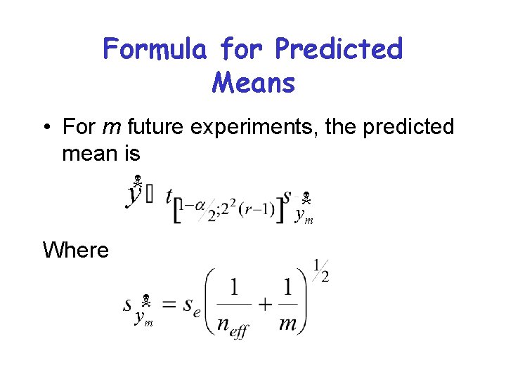
Formula for Predicted Means • For m future experiments, the predicted mean is N y Where N ym

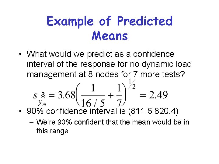
Example of Predicted Means • What would we predict as a confidence interval of the response for no dynamic load management at 8 nodes for 7 more tests? N ym • 90% confidence interval is (811. 6, 820. 4) – We’re 90% confident that the mean would be in this range

Visual Tests for Verifying Assumptions • What assumptions have we been making? – – – Model errors are statistically independent Model errors are additive Errors are normally distributed Errors have constant standard deviation Effects of errors are additive • Which boils down to independent, normally distributed observations with constant variance

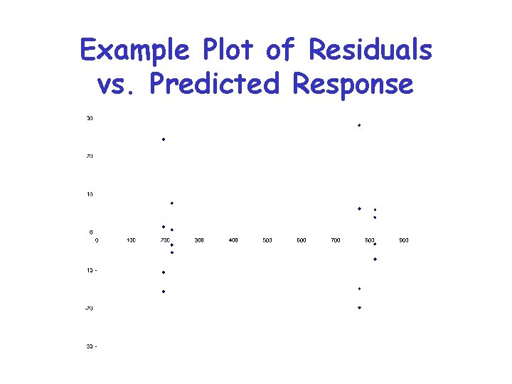
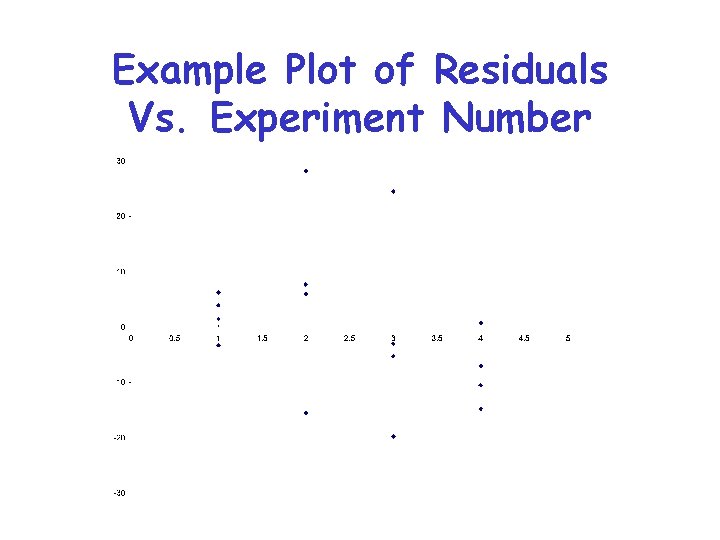
Testing for Independent Errors • Compute residuals and make a scatter plot • Trends indicate a dependence of errors on factor levels – But if residuals order of magnitude below predicted response, trends can be ignored • Sometimes a good idea to plot residuals vs. experiments number

Example Plot of Residuals vs. Predicted Response

Example Plot of Residuals Vs. Experiment Number

Testing for Normally Distributed Errors • As usual, do a quantile-quantile chart – Against the normal distribution • If it’s close to linear, this assumption is good

Quantile-Quantile Plot for Example

Assumption of Constant Variance • Checking homoscedasticity • Go back to the scatter plot and check for an even spread

The Scatter Plot, Again