Density Estimation and MDPs Ronald Parr Stanford University

Density Estimation and MDPs Ronald Parr Stanford University Joint work with Daphne Koller, Andrew Ng (U. C. Berkeley) and Andres Rodriguez

What we aim to do • Plan for/control complex systems • Challenges – very large state spaces – hidden state information • Examples – Drive a car – Ride a bicycle – Operate a factory • Contribution: novel uses of density estimation

Talk Outline • • (PO)MDP overview Traditional (PO)MDP solution methods Density Estimation (PO)MDPs meet density estimation – Reinforcement learning for PO domains – Dynamic programming w/function approx. – Policy search • Experimental Results

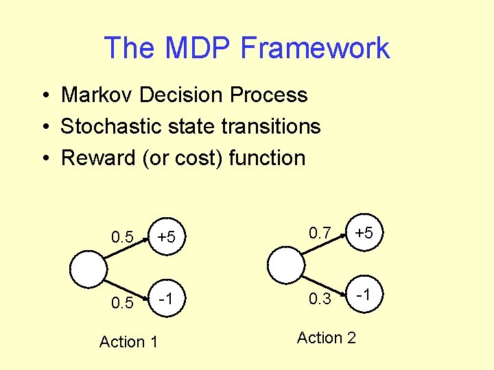
The MDP Framework • Markov Decision Process • Stochastic state transitions • Reward (or cost) function 0. 5 +5 0. 7 +5 0. 5 -1 0. 3 -1 Action 2

MDPs • Uncertain action outcomes • Cost minimization (reward maximization) • Examples – Ride bicycle – Drive car – Operate factory • Assume that full state is known

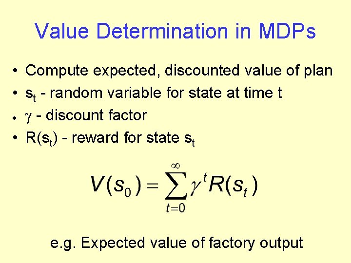
Value Determination in MDPs • Compute expected, discounted value of plan • st - random variable for state at time t g - discount factor • R(st) - reward for state st l e. g. Expected value of factory output

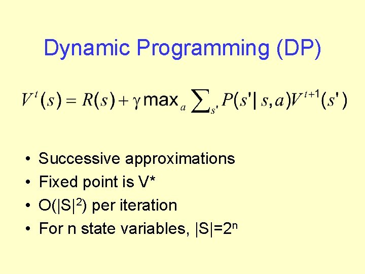
Dynamic Programming (DP) • • Successive approximations Fixed point is V* O(|S|2) per iteration For n state variables, |S|=2 n

Partial Observability • Examples: – road hazards – intentions of other agents – status of equipment • Complication: true state is not known • “state” depends upon history • information state = dist. over true states

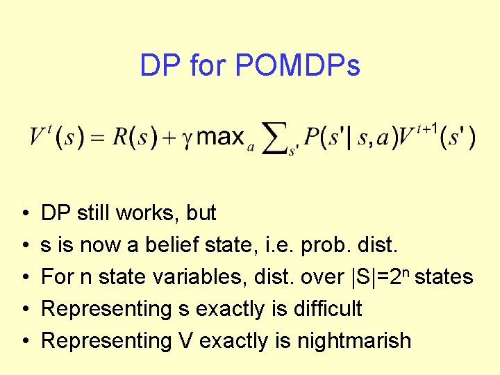
DP for POMDPs • • • DP still works, but s is now a belief state, i. e. prob. dist. For n state variables, dist. over |S|=2 n states Representing s exactly is difficult Representing V exactly is nightmarish

Density Estimation • Efficiently represent dist. over many vars. • Broadly interpreted, includes – Statistical learning • Bayes net learning • Mixture models – Tracking • Kalman filters • DBNs

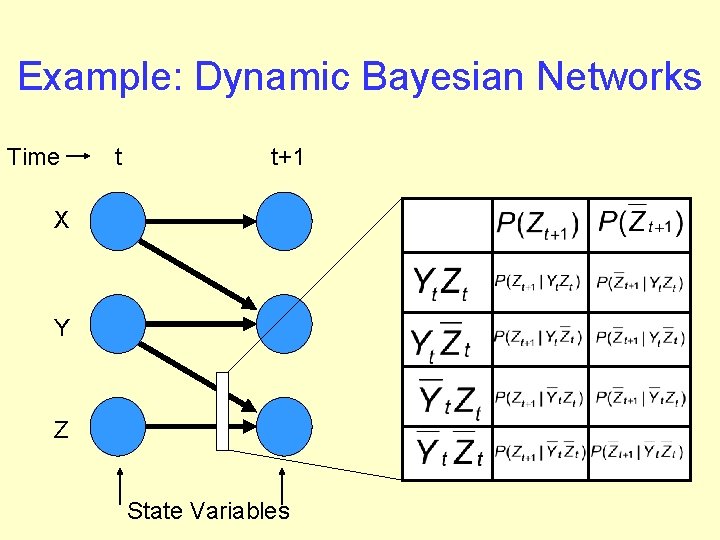
Example: Dynamic Bayesian Networks Time t t+1 X Y Z State Variables

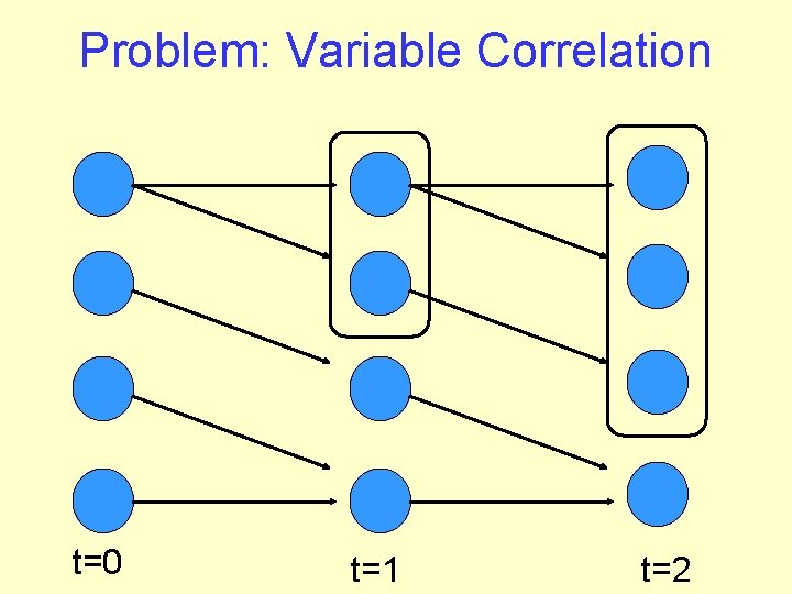
Problem: Variable Correlation t=0 t=1 t=2

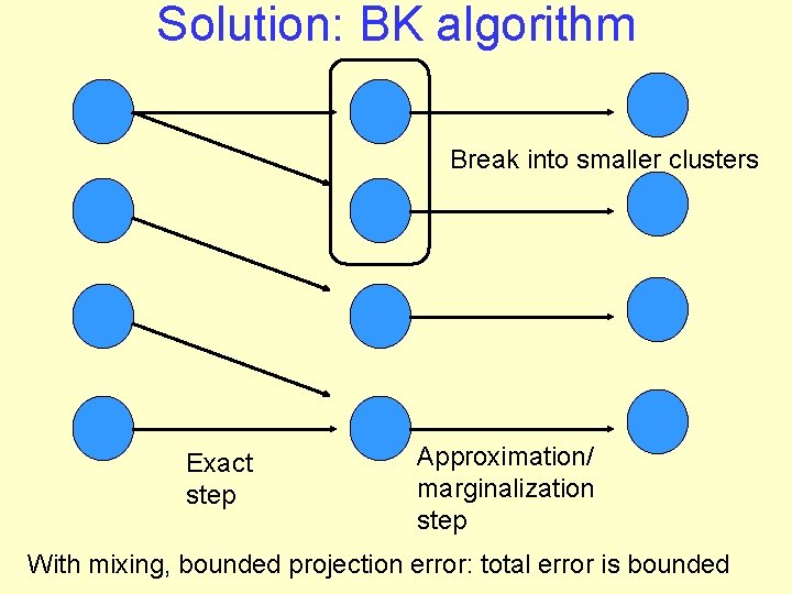
Solution: BK algorithm Break into smaller clusters Exact step Approximation/ marginalization step With mixing, bounded projection error: total error is bounded

Density Estimation meets POMDPs • Problems: – Representing state – Representing value function • Solution: – Use BK algorithm for state estimation – Use reinforcement learning for V (e. g. Parr & Russell 95, Littman et al. 95) – Represent V with neural net • Rodriguez, Parr and Koller, NIPS 99

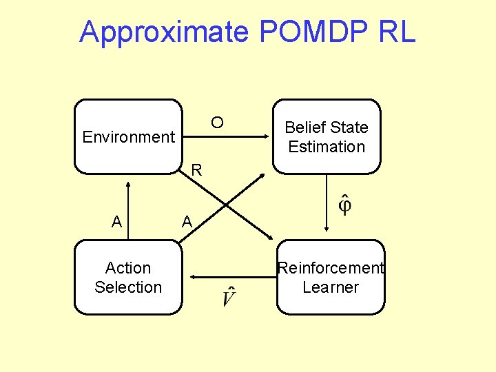
Approximate POMDP RL O Environment Belief State Estimation R A Action Selection A Reinforcement Learner

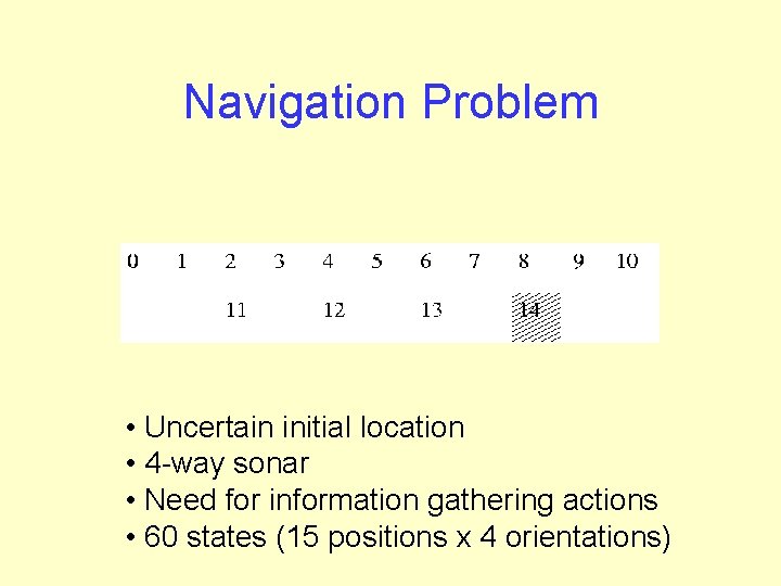
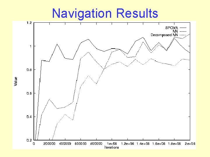
Navigation Problem • Uncertain initial location • 4 -way sonar • Need for information gathering actions • 60 states (15 positions x 4 orientations)

Navigation Results

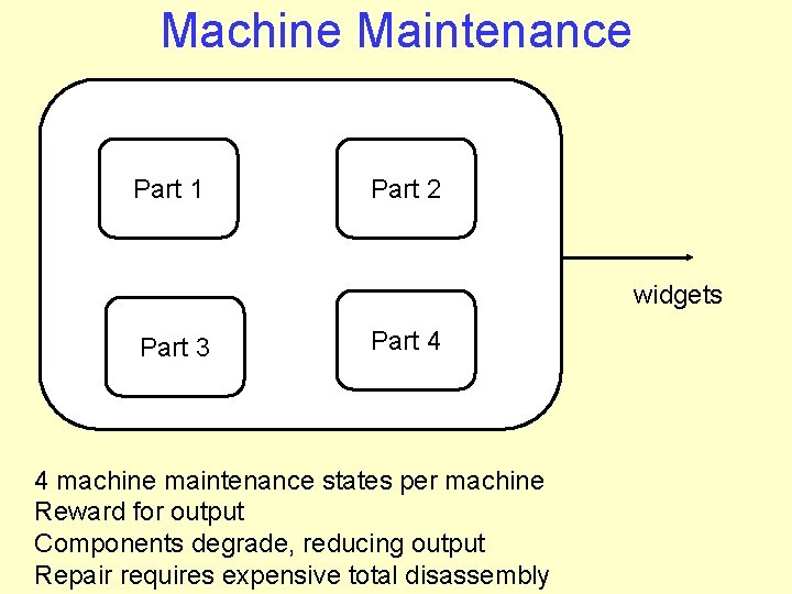
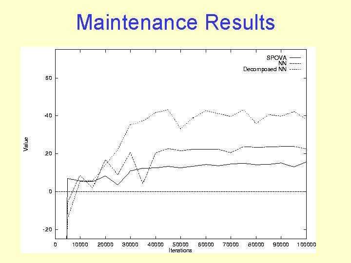
Machine Maintenance Part 1 Part 2 widgets Part 3 Part 4 4 machine maintenance states per machine Reward for output Components degrade, reducing output Repair requires expensive total disassembly

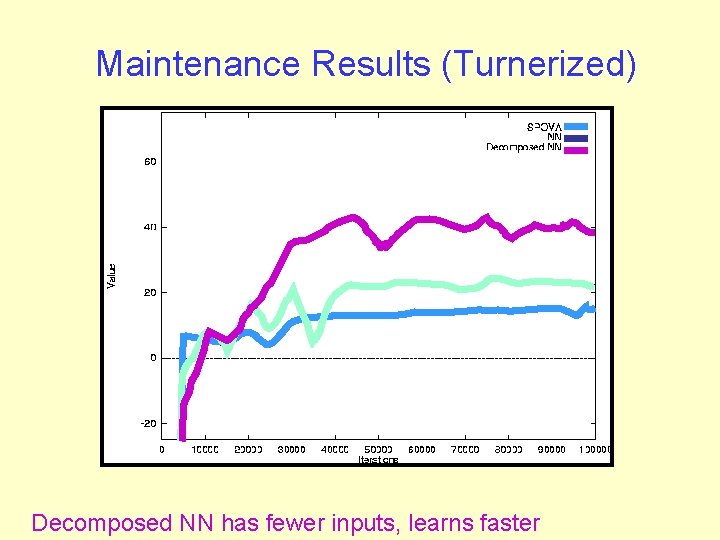
Maintenance Results

Maintenance Results (Turnerized) Decomposed NN has fewer inputs, learns faster

Summary • Advances – Use of factored belief state – Scales POMDP RL to larger state spaces • Limitations – No help with regular MDPs – Can be slow – No convergence guarantees

Goal: DP with guarantees • Focus on value determination in MDPs • Efficient exact DP step • Efficient projection (function approximation) • Non-expansive function approximation (convergence, bounded error)

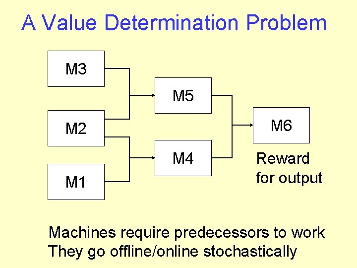
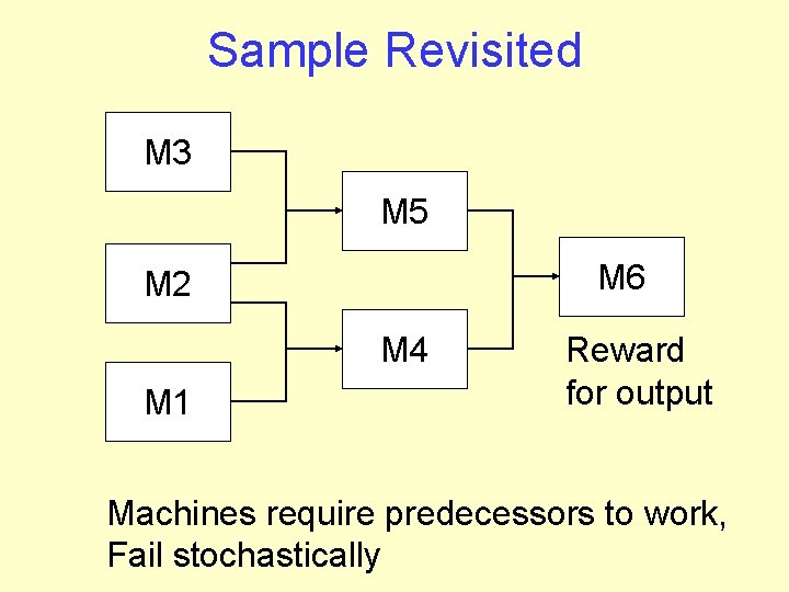
A Value Determination Problem M 3 M 5 M 6 M 2 M 4 M 1 Reward for output Machines require predecessors to work They go offline/online stochastically

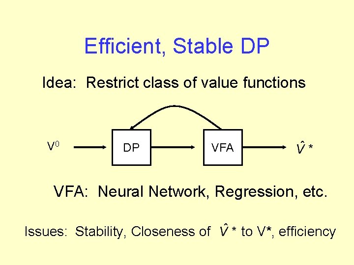
Efficient, Stable DP Idea: Restrict class of value functions V 0 DP VFA: Neural Network, Regression, etc. Issues: Stability, Closeness of to V*, efficiency

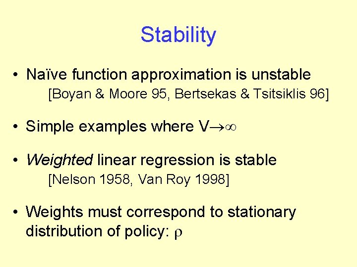
Stability • Naïve function approximation is unstable [Boyan & Moore 95, Bertsekas & Tsitsiklis 96] • Simple examples where V®¥ • Weighted linear regression is stable [Nelson 1958, Van Roy 1998] • Weights must correspond to stationary distribution of policy: r

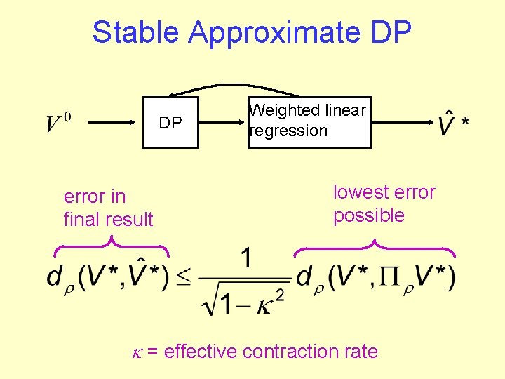
Stable Approximate DP DP error in final result Weighted linear regression lowest error possible = effective contraction rate

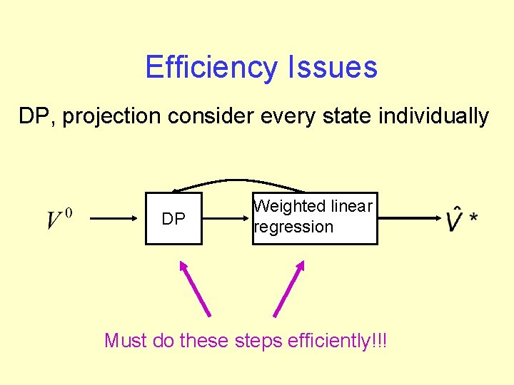
Efficiency Issues DP, projection consider every state individually DP Weighted linear regression Must do these steps efficiently!!!

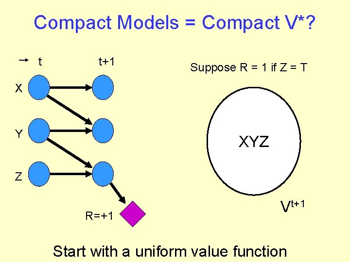
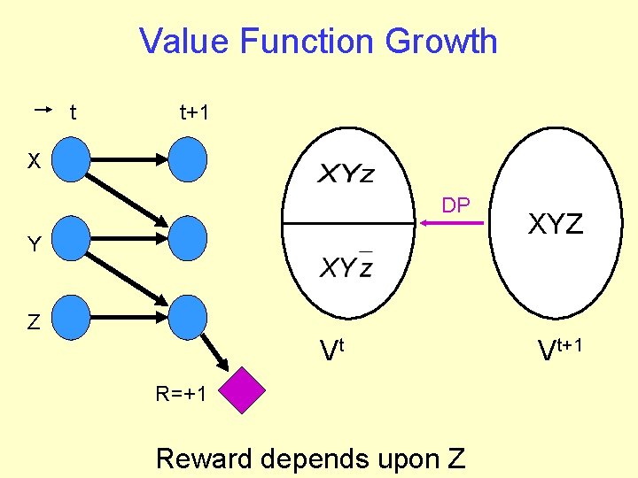
Compact Models = Compact V*? t t+1 Suppose R = 1 if Z = T X Y XYZ Z R=+1 Vt+1 Start with a uniform value function

Value Function Growth t t+1 X DP Y XYZ Z Vt R=+1 Reward depends upon Z Vt+1

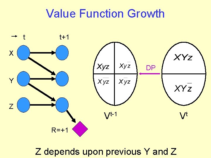
Value Function Growth t t+1 X DP Y Z Vt-1 R=+1 Z depends upon previous Y and Z Vt

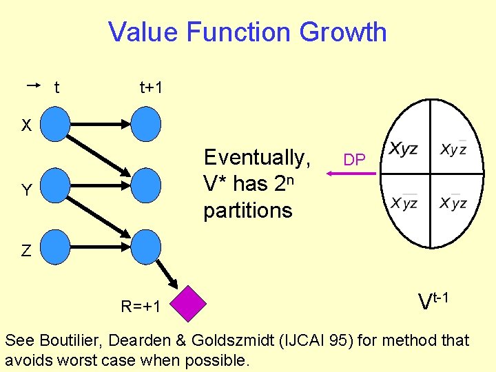
Value Function Growth t t+1 X Eventually, V* has 2 n partitions Y DP Z R=+1 Vt-1 See Boutilier, Dearden & Goldszmidt (IJCAI 95) for method that avoids worst case when possible.

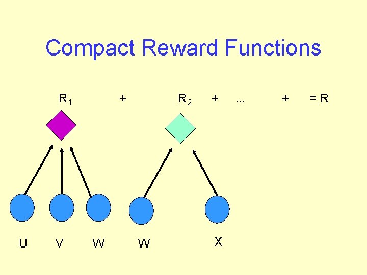
Compact Reward Functions R 1 U V + W R 2 W + X . . . + =R

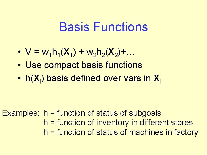
Basis Functions • V = w 1 h 1(X 1) + w 2 h 2(X 2)+… • Use compact basis functions • h(Xi) basis defined over vars in Xi Examples: h = function of status of subgoals h = function of inventory in different stores h = function of status of machines in factory

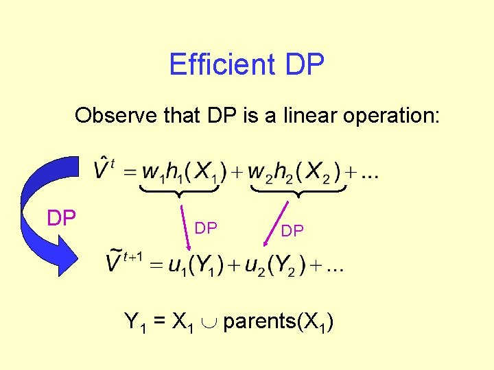
Efficient DP Observe that DP is a linear operation: DP DP DP Y 1 = X 1 È parents(X 1)

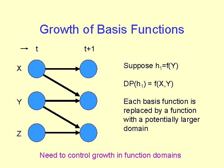
Growth of Basis Functions t X t+1 Suppose h 1=f(Y) DP(h 1) = f(X, Y) Y Z Each basis function is replaced by a function with a potentially larger domain Need to control growth in function domains

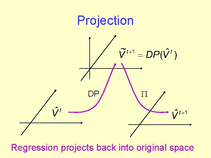
Projection DP P Regression projects back into original space

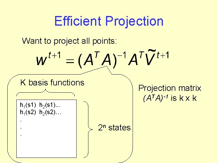
Efficient Projection Want to project all points: K basis functions h 1(s 1) h 2(s 1). . . h 1(s 2) h 2(s 2)…. . . Projection matrix (ATA)-1 is k x k 2 n states

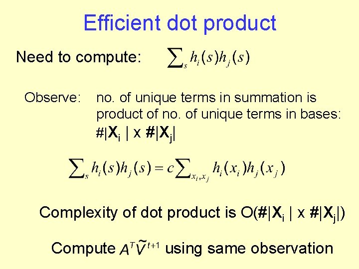
Efficient dot product Need to compute: Observe: no. of unique terms in summation is product of no. of unique terms in bases: #|Xi | x #|Xj| Complexity of dot product is O(#|Xi | x #|Xj|) Compute using same observation

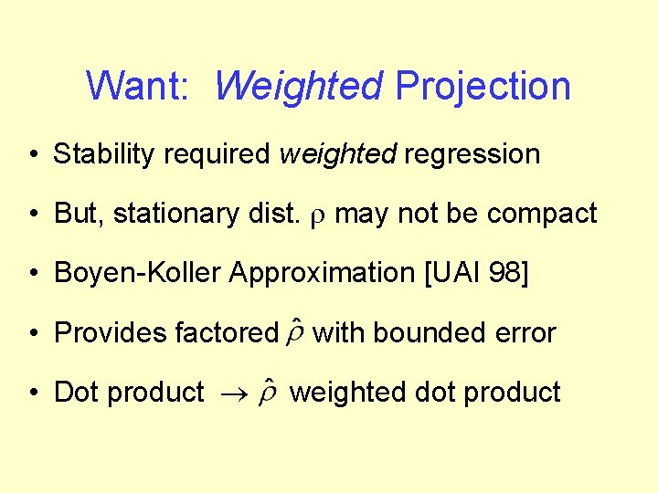
Want: Weighted Projection • Stability required weighted regression • But, stationary dist. r may not be compact • Boyen-Koller Approximation [UAI 98] • Provides factored • Dot product ® with bounded error weighted dot product

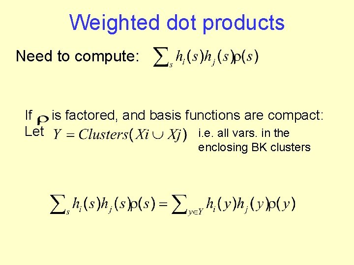
Weighted dot products Need to compute: If is factored, and basis functions are compact: Let i. e. all vars. in the enclosing BK clusters

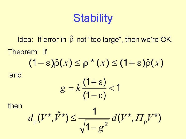
Stability Idea: If error in Theorem: If and then not “too large”, then we’re OK.

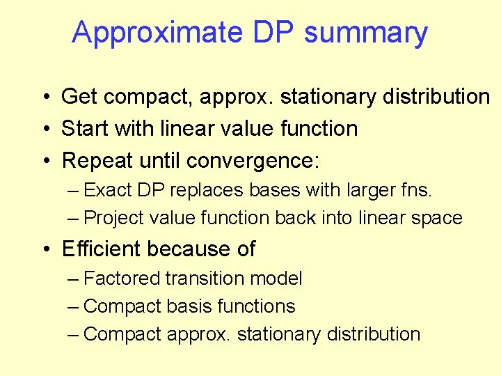
Approximate DP summary • Get compact, approx. stationary distribution • Start with linear value function • Repeat until convergence: – Exact DP replaces bases with larger fns. – Project value function back into linear space • Efficient because of – Factored transition model – Compact basis functions – Compact approx. stationary distribution

Sample Revisited M 3 M 5 M 6 M 2 M 4 M 1 Reward for output Machines require predecessors to work, Fail stochastically

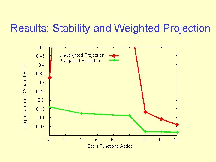
Results: Stability and Weighted Projection 0. 5 Unweighted Projection Weighted Sum of Squared Errors 0. 45 0. 4 0. 35 0. 3 0. 25 0. 2 0. 15 0. 1 0. 05 0 2 3 4 5 6 7 Basis Functions Added 8 9 10

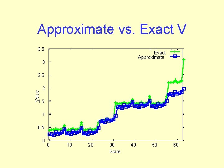
Approximate vs. Exact V 3. 5 Exact Approximate 3 Value 2. 5 2 1. 5 1 0. 5 0 0 10 20 30 State 40 50 60

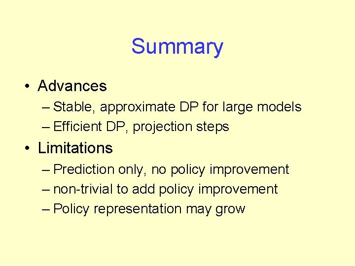
Summary • Advances – Stable, approximate DP for large models – Efficient DP, projection steps • Limitations – Prediction only, no policy improvement – non-trivial to add policy improvement – Policy representation may grow

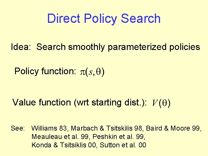
Direct Policy Search Idea: Search smoothly parameterized policies Policy function: Value function (wrt starting dist. ): See: Williams 83, Marbach & Tsitskilis 98, Baird & Moore 99, Meauleau et al. 99, Peshkin et al. 99, Konda & Tsitsiklis 00, Sutton et al. 00

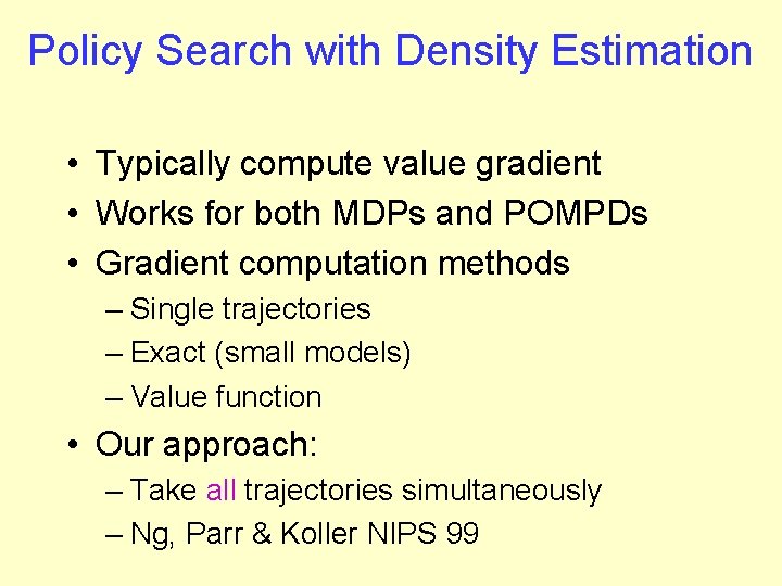
Policy Search with Density Estimation • Typically compute value gradient • Works for both MDPs and POMPDs • Gradient computation methods – Single trajectories – Exact (small models) – Value function • Our approach: – Take all trajectories simultaneously – Ng, Parr & Koller NIPS 99

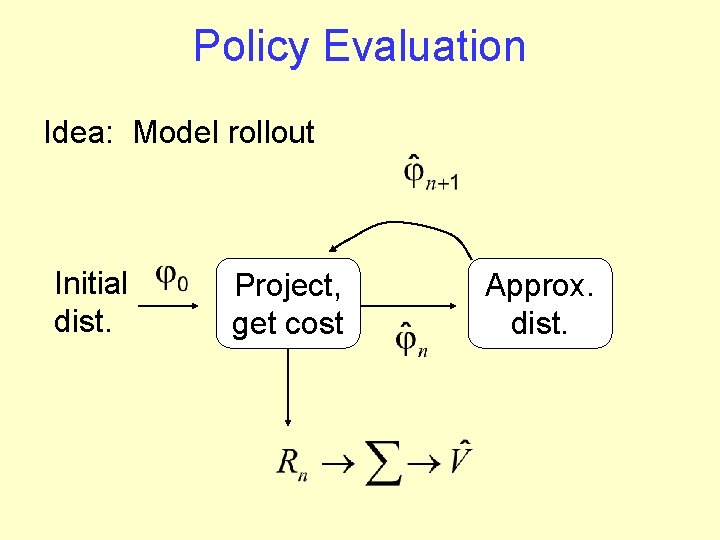
Policy Evaluation Idea: Model rollout Initial dist. Project, get cost Approx. dist.

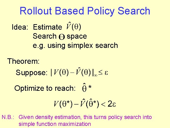
Rollout Based Policy Search Idea: Estimate Search space e. g. using simplex search Theorem: Suppose: Optimize to reach: N. B. : Given density estimation, this turns policy search into simple function maximization

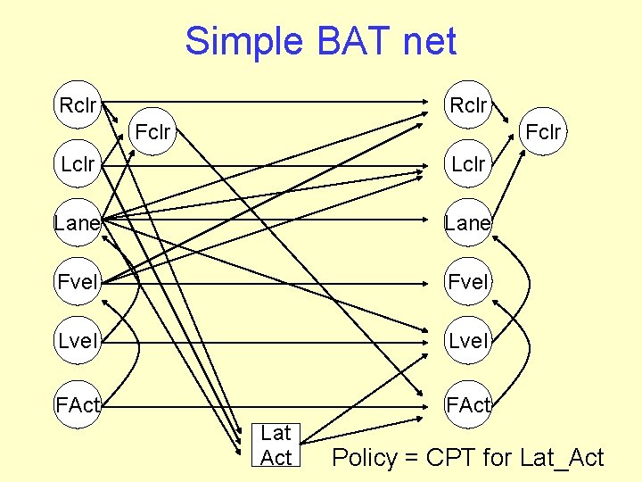
Simple BAT net Rclr Fclr Lclr Lane Fvel Lvel FAct Lat Act Policy = CPT for Lat_Act

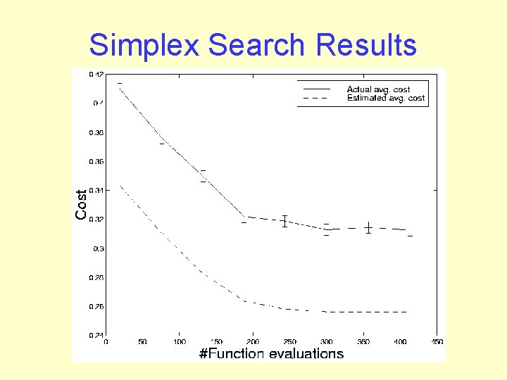
Simplex Search Results

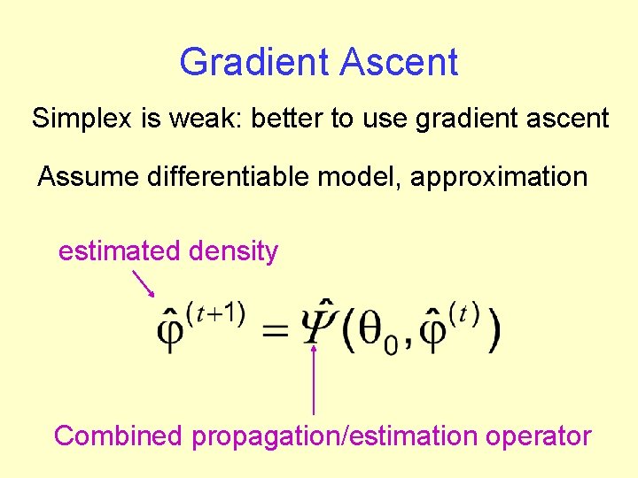
Gradient Ascent Simplex is weak: better to use gradient ascent Assume differentiable model, approximation estimated density Combined propagation/estimation operator

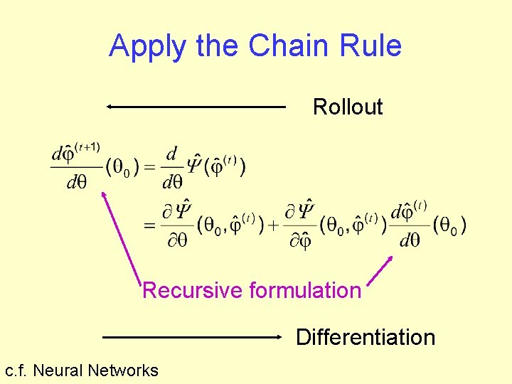
Apply the Chain Rule Rollout Recursive formulation Differentiation c. f. Neural Networks

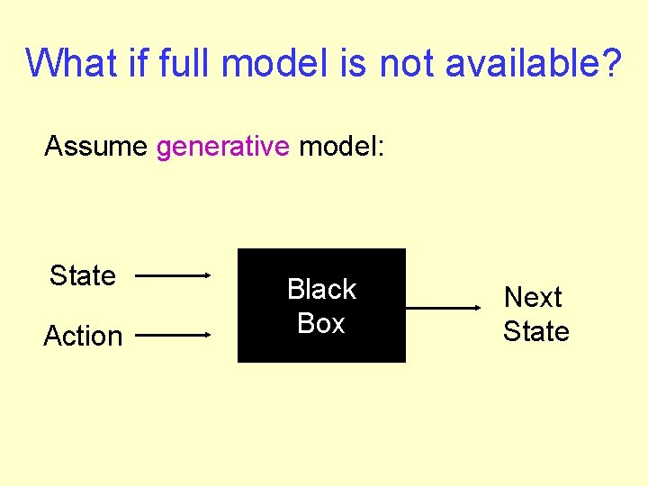
What if full model is not available? Assume generative model: State Action Black Box Next State

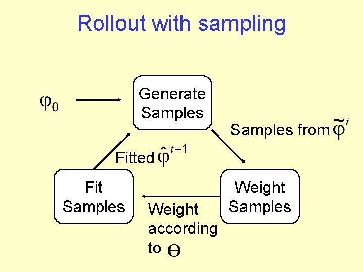
Rollout with sampling Generate Samples from Fitted Fit Samples Weight according to Weight Samples

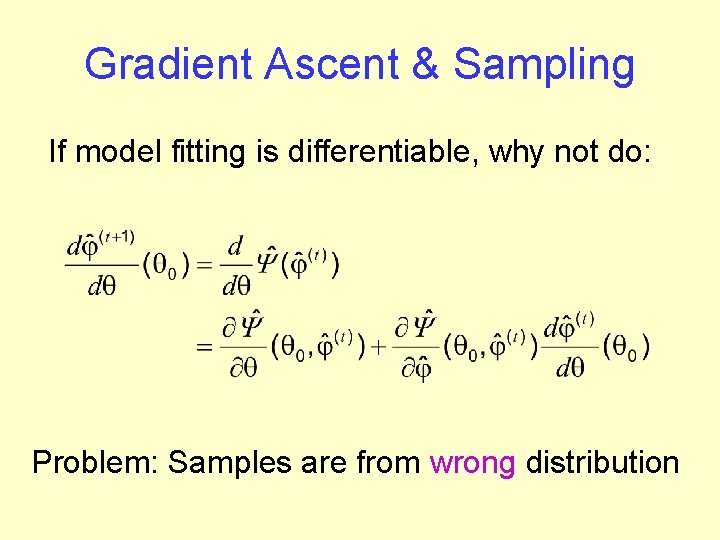
Gradient Ascent & Sampling If model fitting is differentiable, why not do: Problem: Samples are from wrong distribution

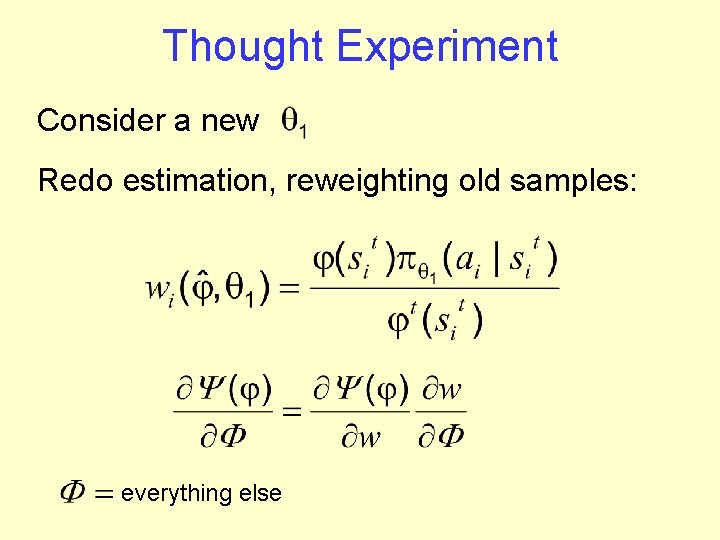
Thought Experiment Consider a new Redo estimation, reweighting old samples: everything else

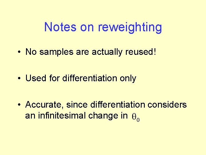
Notes on reweighting • No samples are actually reused! • Used for differentiation only • Accurate, since differentiation considers an infinitesimal change in

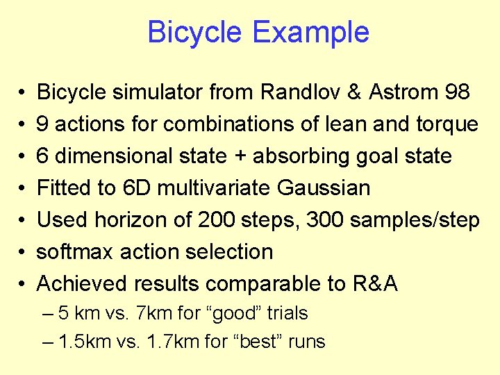
Bicycle Example • • Bicycle simulator from Randlov & Astrom 98 9 actions for combinations of lean and torque 6 dimensional state + absorbing goal state Fitted to 6 D multivariate Gaussian Used horizon of 200 steps, 300 samples/step softmax action selection Achieved results comparable to R&A – 5 km vs. 7 km for “good” trials – 1. 5 km vs. 1. 7 km for “best” runs

Conclusions • 3 new uses for density estimation in (PO)MDPs • POMDP RL – Function approx. with density estimation • Structured MDPs – Value determination with guarantees • Policy search – Search space of parameterized policies