Stanford CS 223 B Computer Vision Winter 2006

Stanford CS 223 B Computer Vision, Winter 2006 Stereo Lecture 6 Stereo II Professor Sebastian Thrun CAs: Dan Maynes-Aminzade, Mitul Saha, Greg Corrado

Stereo Vision: Outline n n n n Basic Equations Epipolar Geometry Image Rectification Reconstruction Correspondence Active Range Imaging Technology Dense and Layered Stereo Smoothing With Markov Random Fields Sebastian Thrun Stanford University CS 223 B Computer Vision

A Last Word on Preprocessing…. Sebastian Thrun Stanford University CS 223 B Computer Vision

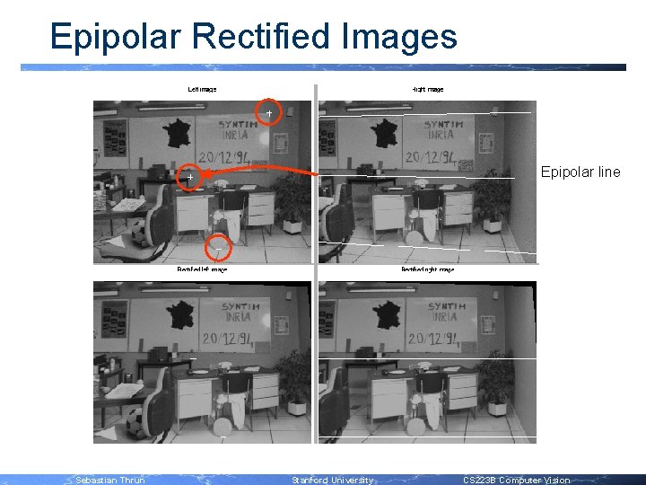
Epipolar Rectified Images Epipolar line Sebastian Thrun Stanford University CS 223 B Computer Vision

Epipolar Rectified Images Source: A. Fusiello, Verona, 2000] Sebastian Thrun Stanford University CS 223 B Computer Vision

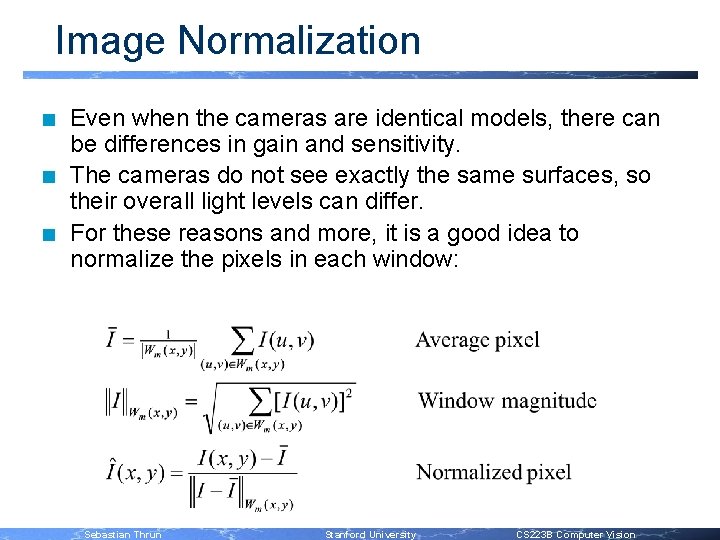
Image Normalization n Even when the cameras are identical models, there can be differences in gain and sensitivity. The cameras do not see exactly the same surfaces, so their overall light levels can differ. For these reasons and more, it is a good idea to normalize the pixels in each window: Sebastian Thrun Stanford University CS 223 B Computer Vision

Stereo Vision: Outline n n n n Basic Equations Epipolar Geometry Image Rectification Reconstruction Correspondence Active Range Imaging Technology Dense and Layered Stereo Smoothing With Markov Random Fields Sebastian Thrun Stanford University CS 223 B Computer Vision

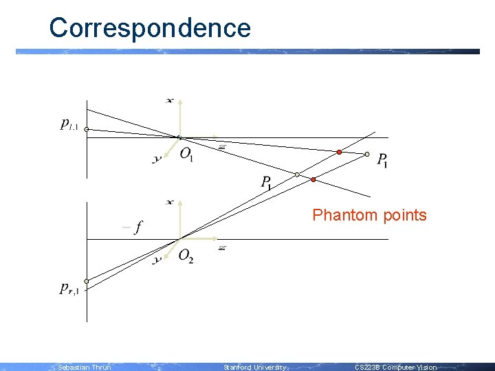
Correspondence Phantom points Sebastian Thrun Stanford University CS 223 B Computer Vision

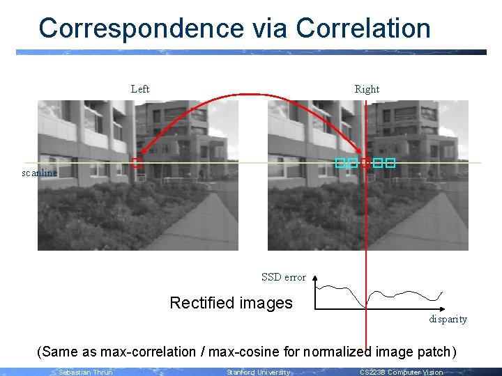
Correspondence via Correlation Left Right scanline SSD error Rectified images disparity (Same as max-correlation / max-cosine for normalized image patch) Sebastian Thrun Stanford University CS 223 B Computer Vision

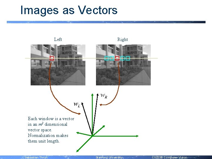
Images as Vectors Left Right Each window is a vector in an m 2 dimensional vector space. Normalization makes them unit length. Sebastian Thrun Stanford University CS 223 B Computer Vision

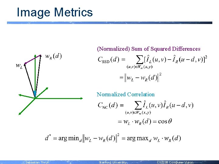
Image Metrics (Normalized) Sum of Squared Differences Normalized Correlation Sebastian Thrun Stanford University CS 223 B Computer Vision

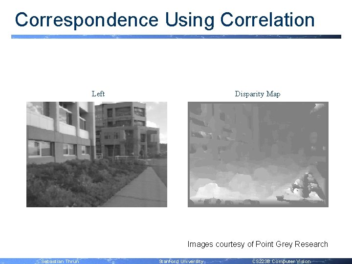
Correspondence Using Correlation Left Disparity Map Images courtesy of Point Grey Research Sebastian Thrun Stanford University CS 223 B Computer Vision

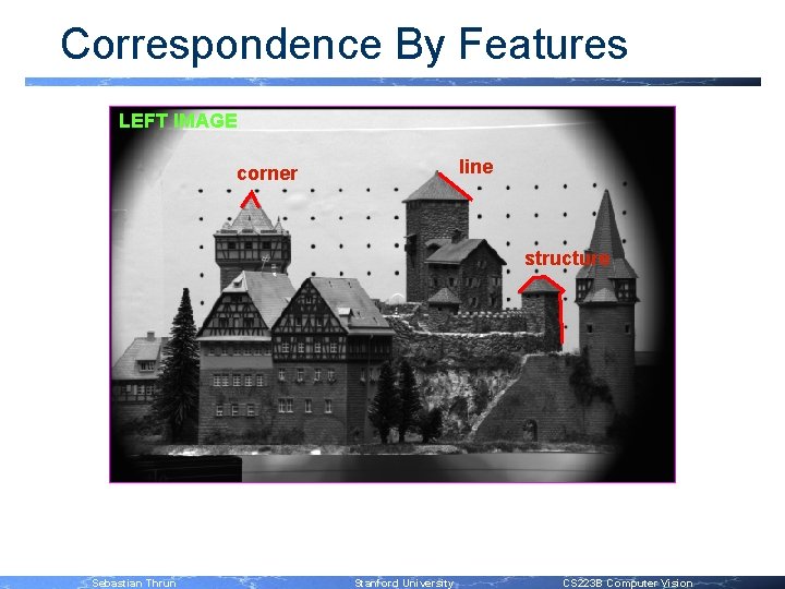
Correspondence By Features LEFT IMAGE line corner structure Sebastian Thrun Stanford University CS 223 B Computer Vision

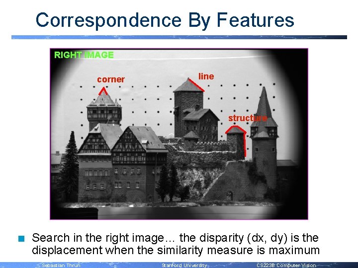
Correspondence By Features RIGHT IMAGE corner line structure n Search in the right image… the disparity (dx, dy) is the displacement when the similarity measure is maximum Sebastian Thrun Stanford University CS 223 B Computer Vision

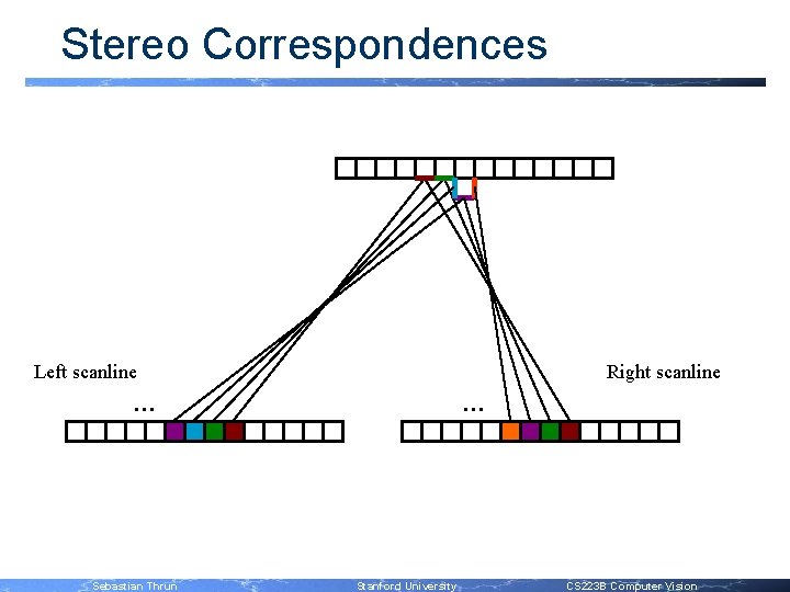
Stereo Correspondences Left scanline Right scanline … Sebastian Thrun … Stanford University CS 223 B Computer Vision

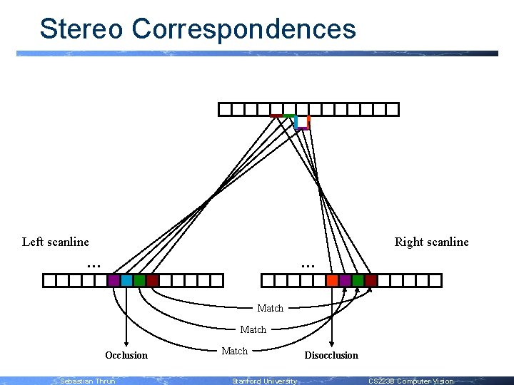
Stereo Correspondences Left scanline Right scanline … … Match Occlusion Sebastian Thrun Match Stanford University Disocclusion CS 223 B Computer Vision

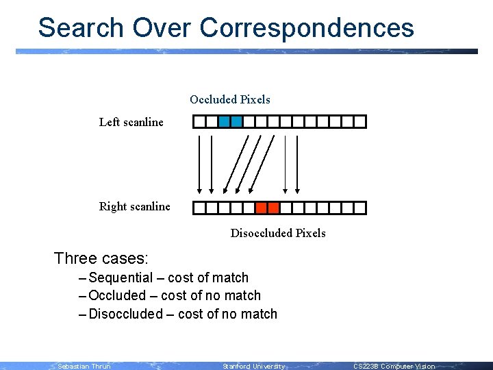
Search Over Correspondences Occluded Pixels Left scanline Right scanline Disoccluded Pixels Three cases: – Sequential – cost of match – Occluded – cost of no match – Disoccluded – cost of no match Sebastian Thrun Stanford University CS 223 B Computer Vision

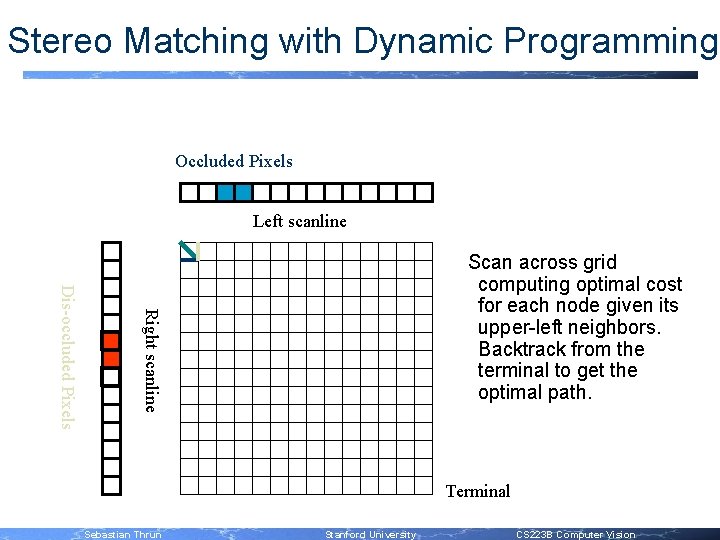
Stereo Matching with Dynamic Programming Occluded Pixels Left scanline Right scanline Dis-occluded Pixels Scan across grid computing optimal cost for each node given its upper-left neighbors. Backtrack from the terminal to get the optimal path. Terminal Sebastian Thrun Stanford University CS 223 B Computer Vision

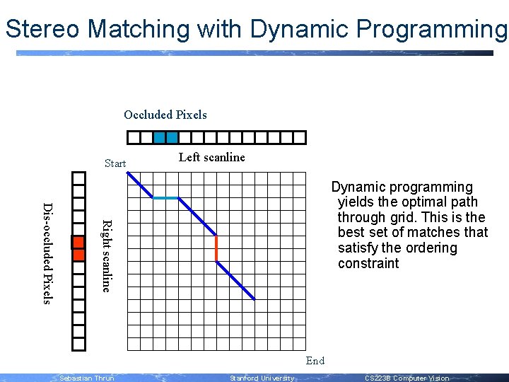
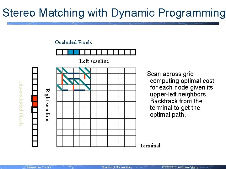
Stereo Matching with Dynamic Programming Occluded Pixels Start Left scanline Right scanline Dis-occluded Pixels Dynamic programming yields the optimal path through grid. This is the best set of matches that satisfy the ordering constraint End Sebastian Thrun Stanford University CS 223 B Computer Vision

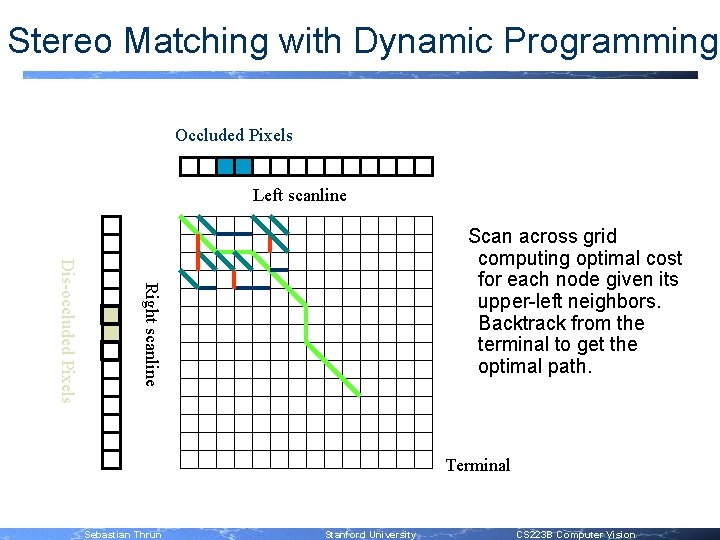
Stereo Matching with Dynamic Programming Occluded Pixels Left scanline Right scanline Dis-occluded Pixels Scan across grid computing optimal cost for each node given its upper-left neighbors. Backtrack from the terminal to get the optimal path. Terminal Sebastian Thrun Stanford University CS 223 B Computer Vision

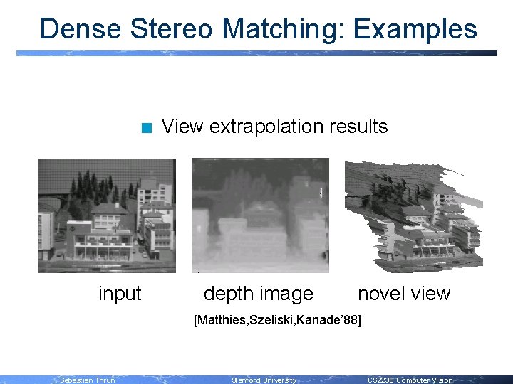
Dense Stereo Matching: Examples n input View extrapolation results depth image novel view [Matthies, Szeliski, Kanade’ 88] Sebastian Thrun Stanford University CS 223 B Computer Vision

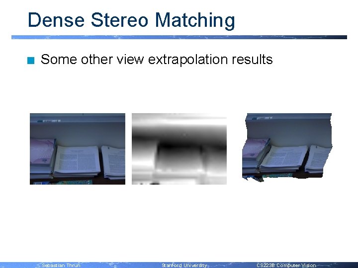
Dense Stereo Matching n Some other view extrapolation results input Sebastian Thrun depth image Stanford University novel view CS 223 B Computer Vision

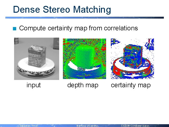
Dense Stereo Matching n Compute certainty map from correlations input Sebastian Thrun depth map Stanford University certainty map CS 223 B Computer Vision

DP for Correspondence n n Does this always work? When would it fail? – Failure Example 1 – Failure Example 2 – Failure Example 3 Sebastian Thrun Stanford University CS 223 B Computer Vision

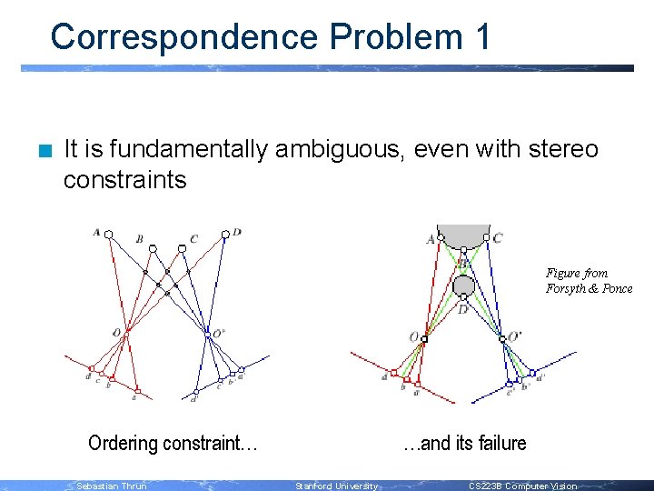
Correspondence Problem 1 n It is fundamentally ambiguous, even with stereo constraints Figure from Forsyth & Ponce Ordering constraint… Sebastian Thrun …and its failure Stanford University CS 223 B Computer Vision

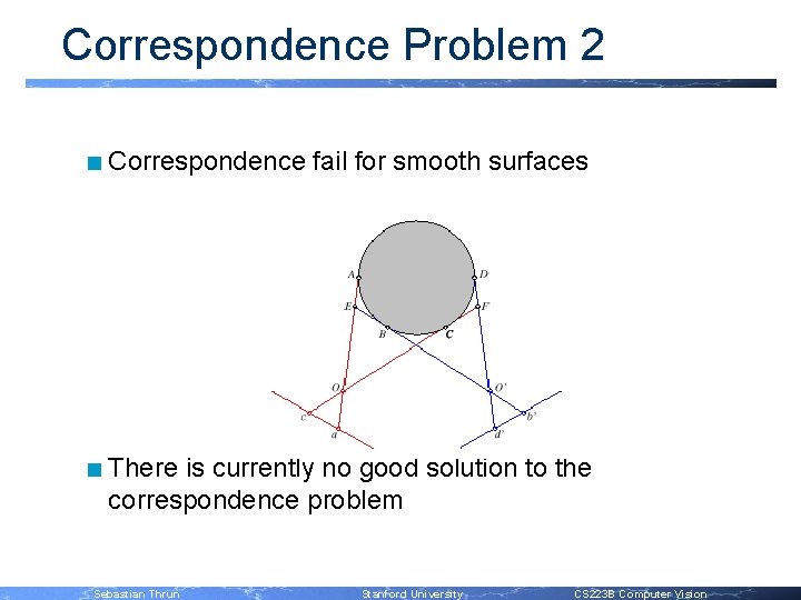
Correspondence Problem 2 n Correspondence fail for smooth surfaces n There is currently no good solution to the correspondence problem Sebastian Thrun Stanford University CS 223 B Computer Vision

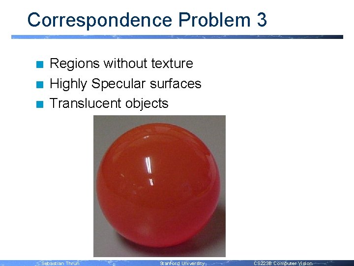
Correspondence Problem 3 n n n Regions without texture Highly Specular surfaces Translucent objects Sebastian Thrun Stanford University CS 223 B Computer Vision

Stereo Vision: Outline n n n n Basic Equations Epipolar Geometry Image Rectification Reconstruction Correspondence Active Range Imaging Technology Dense and Layered Stereo Smoothing With Markov Random Fields Sebastian Thrun Stanford University CS 223 B Computer Vision

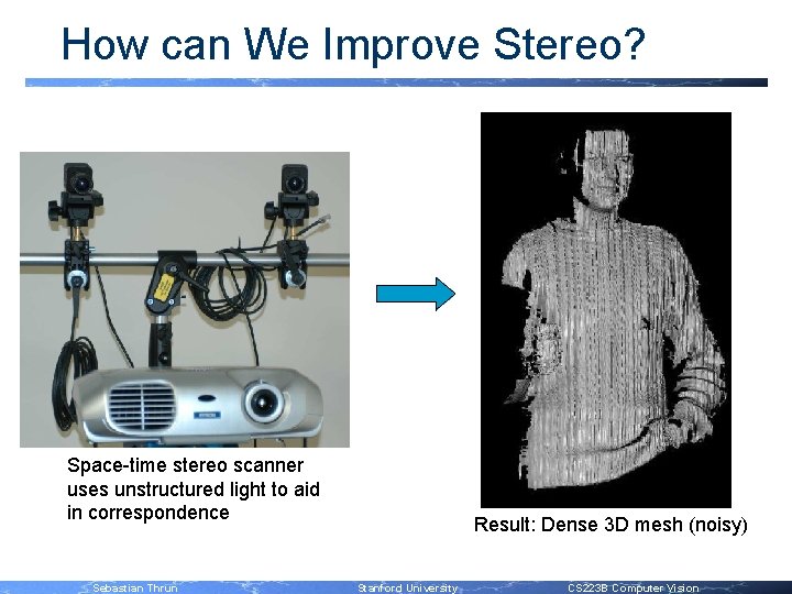
How can We Improve Stereo? Space-time stereo scanner uses unstructured light to aid in correspondence Sebastian Thrun Result: Dense 3 D mesh (noisy) Stanford University CS 223 B Computer Vision

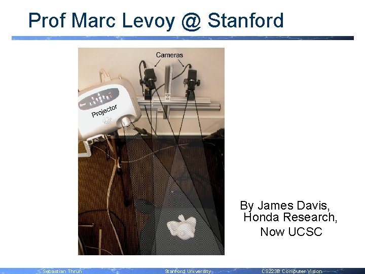
Prof Marc Levoy @ Stanford By James Davis, Honda Research, Now UCSC Sebastian Thrun Stanford University CS 223 B Computer Vision

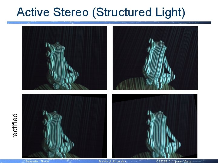
rectified Active Stereo (Structured Light) Sebastian Thrun Stanford University CS 223 B Computer Vision

Structured Light: 3 -D Result 3 D Snapshot 3 D Model By James Davis, Honda Research Sebastian Thrun Stanford University CS 223 B Computer Vision

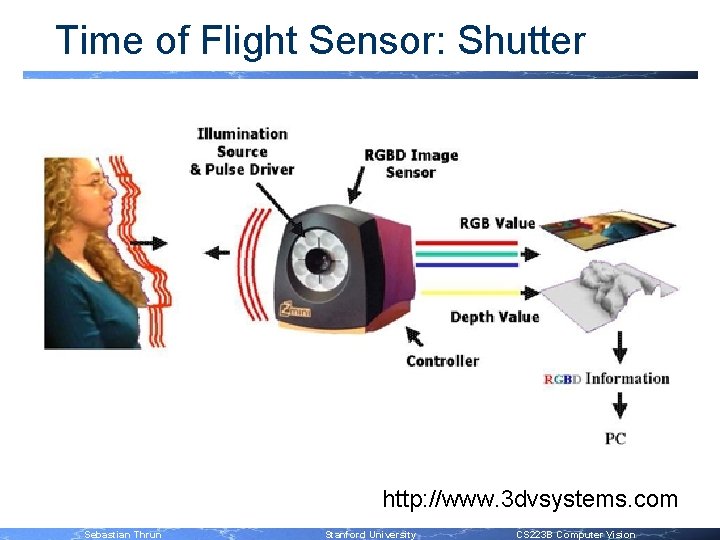
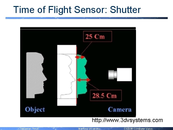
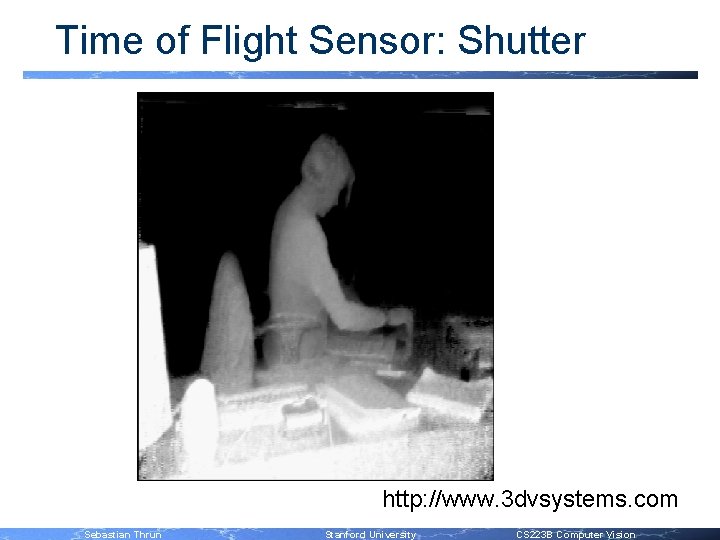
Time of Flight Sensor: Shutter http: //www. 3 dvsystems. com Sebastian Thrun Stanford University CS 223 B Computer Vision

Stereo Vision: Outline n n n n Basic Equations Epipolar Geometry Image Rectification Reconstruction Correspondence Active Range Imaging Technology Layered Stereo Smoothing With Markov Random Fields Sebastian Thrun Stanford University CS 223 B Computer Vision

Disclaimer n The Following Material Shall Not Be Required For the Midterm Exam Sebastian Thrun Stanford University CS 223 B Computer Vision

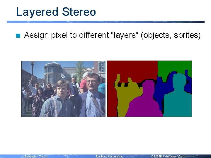
Layered Stereo n Assign pixel to different “layers” (objects, sprites) Sebastian Thrun Stanford University CS 223 B Computer Vision

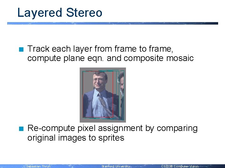
Layered Stereo n Track each layer from frame to frame, compute plane eqn. and composite mosaic n Re-compute pixel assignment by comparing original images to sprites Sebastian Thrun Stanford University CS 223 B Computer Vision

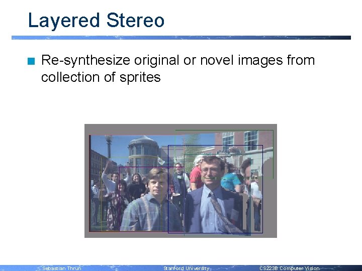
Layered Stereo n Re-synthesize original or novel images from collection of sprites Sebastian Thrun Stanford University CS 223 B Computer Vision

Layered Stereo n Advantages: – can represent occluded regions – can represent transparent and border (mixed) pixels (sprites have alpha value per pixel) – works on texture-less interior regions n Limitations: – fails for high depth-complexity scenes Sebastian Thrun Stanford University CS 223 B Computer Vision

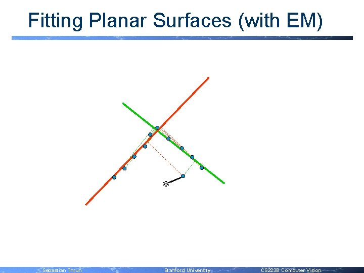
Fitting Planar Surfaces (with EM) * Sebastian Thrun Stanford University * CS 223 B Computer Vision

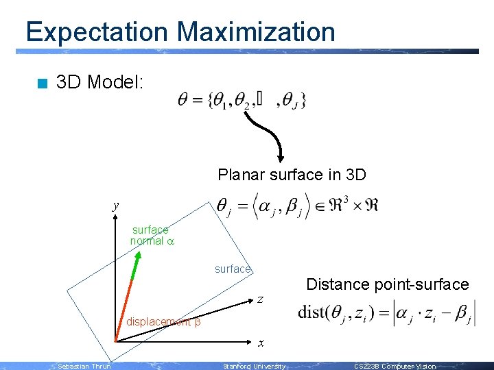
Expectation Maximization n 3 D Model: Planar surface in 3 D y surface normal a surface z Distance point-surface displacement b x Sebastian Thrun Stanford University CS 223 B Computer Vision

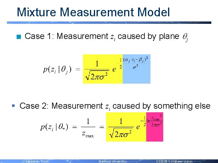
Mixture Measurement Model n Case 1: Measurement zi caused by plane qj § Case 2: Measurement zi caused by something else Sebastian Thrun Stanford University CS 223 B Computer Vision

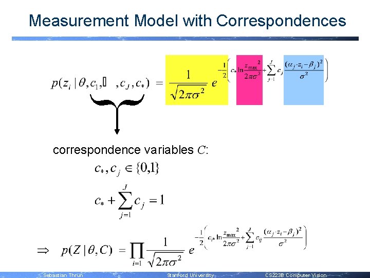
Measurement Model with Correspondences } correspondence variables C: Sebastian Thrun Stanford University CS 223 B Computer Vision

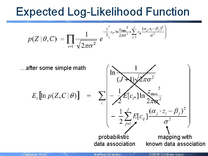
Expected Log-Likelihood Function …after some simple math probabilistic data association Sebastian Thrun Stanford University mapping with known data association CS 223 B Computer Vision

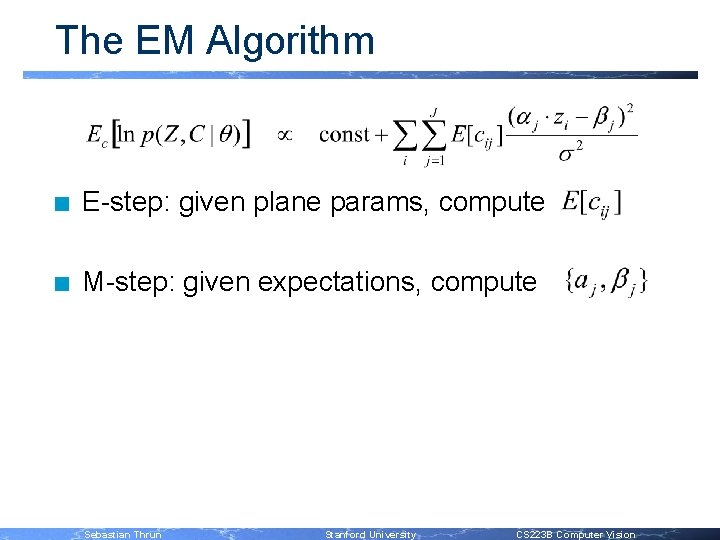
The EM Algorithm n E-step: given plane params, compute n M-step: given expectations, compute Sebastian Thrun Stanford University CS 223 B Computer Vision

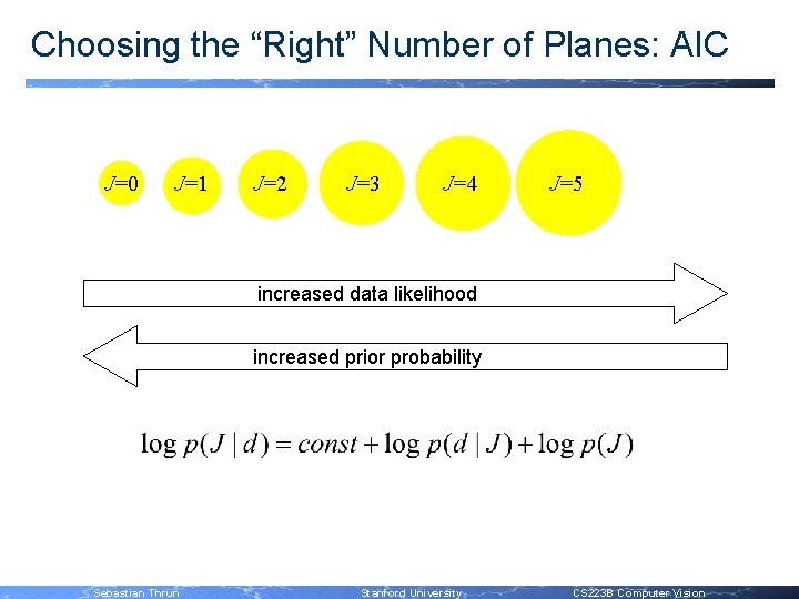
Choosing the “Right” Number of Planes: AIC J=0 J=1 J=2 J=3 J=4 J=5 increased data likelihood increased prior probability Sebastian Thrun Stanford University CS 223 B Computer Vision

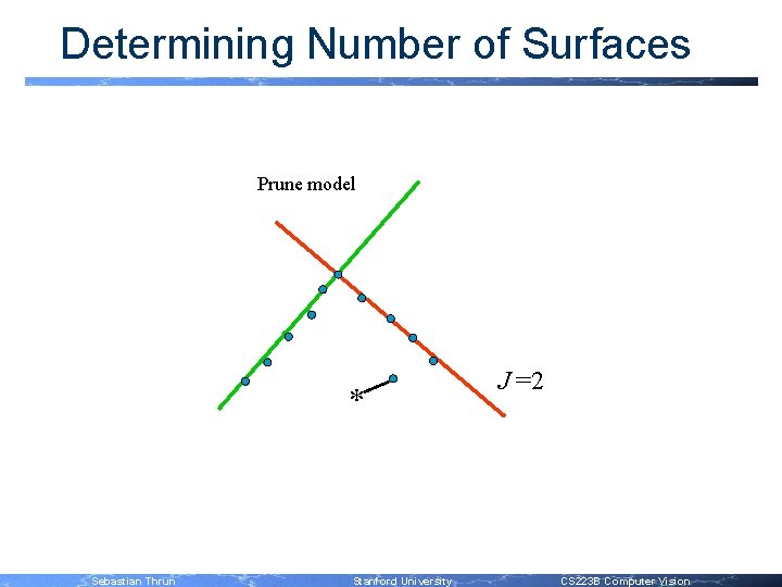
Determining Number of Surfaces Add Firstmodel Prune E/M M-step E-Steps components model component * * Sebastian Thrun J =2 =1 =3 * Stanford University CS 223 B Computer Vision

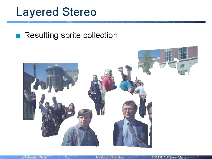
Layered Stereo n Resulting sprite collection Sebastian Thrun Stanford University CS 223 B Computer Vision

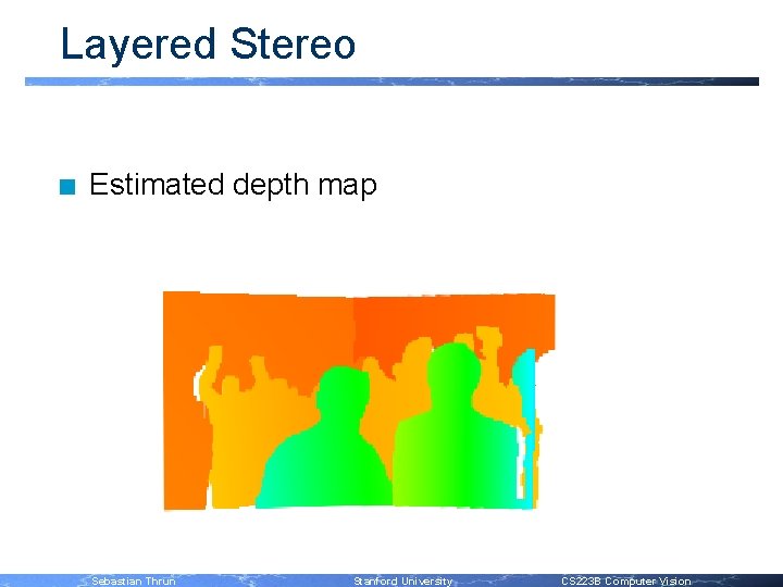
Layered Stereo n Estimated depth map Sebastian Thrun Stanford University CS 223 B Computer Vision

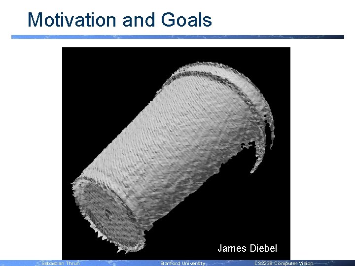
Stereo Vision: Outline n n n n Basic Equations Epipolar Geometry Image Rectification Reconstruction Correspondence Active Range Imaging Technology Dense and Layered Stereo Smoothing With Markov Random Fields Sebastian Thrun Stanford University CS 223 B Computer Vision

Motivation and Goals James Diebel Sebastian Thrun Stanford University CS 223 B Computer Vision

Network of Constraints (Markov Random Field) James Diebel Sebastian Thrun Stanford University CS 223 B Computer Vision

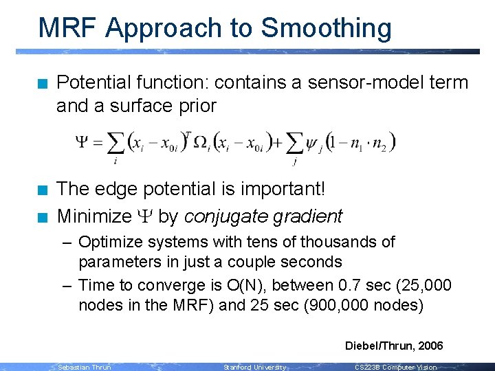
MRF Approach to Smoothing n Potential function: contains a sensor-model term and a surface prior n The edge potential is important! Minimize by conjugate gradient n – Optimize systems with tens of thousands of parameters in just a couple seconds – Time to converge is O(N), between 0. 7 sec (25, 000 nodes in the MRF) and 25 sec (900, 000 nodes) Diebel/Thrun, 2006 Sebastian Thrun Stanford University CS 223 B Computer Vision

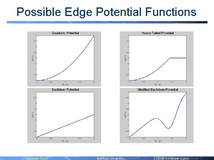
Possible Edge Potential Functions Sebastian Thrun Stanford University CS 223 B Computer Vision

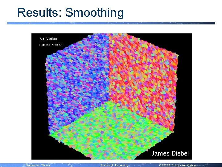
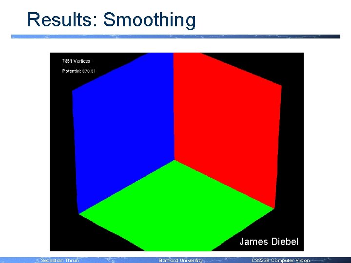
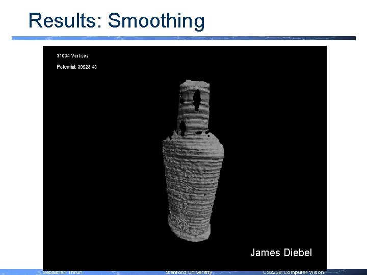
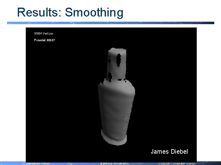
Results: Smoothing James Diebel Sebastian Thrun Stanford University CS 223 B Computer Vision

Movies… Movies in Windows Media Player Sebastian Thrun Stanford University CS 223 B Computer Vision

Stereo Vision: Outline n n n n Basic Equations Epipolar Geometry Image Rectification Reconstruction Correspondence Active Range Imaging Technology Dense and Layered Stereo Smoothing With Markov Random Fields Sebastian Thrun Stanford University CS 223 B Computer Vision