Dealing with Missing Values Dealing with Missing Values

Dealing with Missing Values

Dealing with Missing Values 1. 2. 3. 4. 5. 6. Introduction Assumptions and Missing Data Mechanisms Simple Approaches to Missing Data Maximum Likelihood Imputation Methods Machine Learning Based Methods Experimental Comparative Analysis

Dealing with Missing Values 1. 2. 3. 4. 5. 6. Introduction Assumptions and Missing Data Mechanisms Simple Approaches to Missing Data Maximum Likelihood Imputation Methods Machine Learning Based Methods Experimental Comparative Analysis

Introduction • A missing value (MV) is just a value for attribute that was not introduced or was lost in the recording process: – Equipment errors – Manual data entry procedures – Incorrect measurements

Introduction • MVs make performing data analysis difficult • Also inappropriate handling of the MVs in the analysis may introduce bias and can result in misleading conclusions • Problems are usually associated with MVs: 1. loss of efficiency; 2. complications in handling and analyzing the data; 3. bias resulting from differences between missing and complete data.

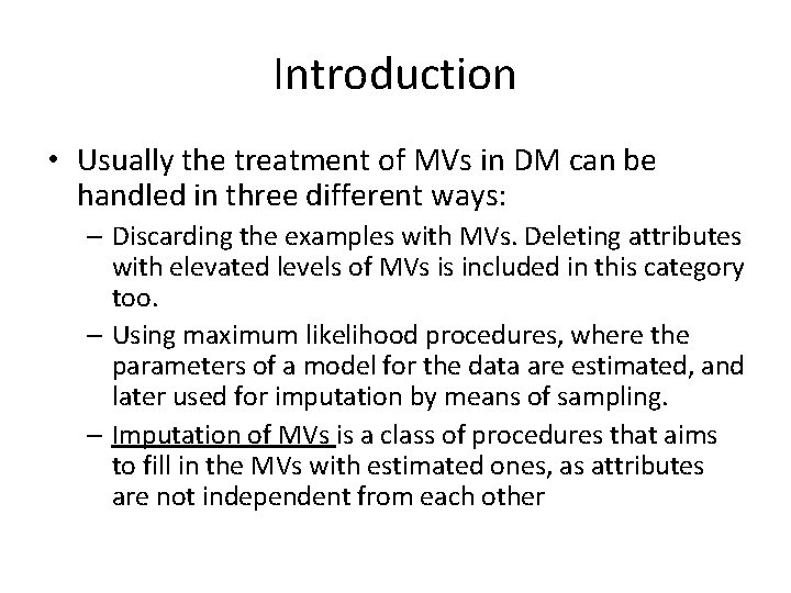
Introduction • Usually the treatment of MVs in DM can be handled in three different ways: – Discarding the examples with MVs. Deleting attributes with elevated levels of MVs is included in this category too. – Using maximum likelihood procedures, where the parameters of a model for the data are estimated, and later used for imputation by means of sampling. – Imputation of MVs is a class of procedures that aims to fill in the MVs with estimated ones, as attributes are not independent from each other

Dealing with Missing Values 1. 2. 3. 4. 5. 6. Introduction Assumptions and Missing Data Mechanisms Simple Approaches to Missing Data Maximum Likelihood Imputation Methods Machine Learning Based Methods Experimental Comparative Analysis

Assumptions and Missing Data Mechanisms • It is important to categorize the mechanisms which lead to the introduction of MVs • The assumptions we make about the missingness mechanism can affect which treatment method could be correctly applied, if any

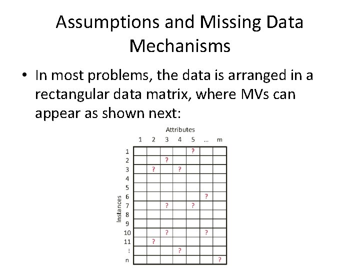
Assumptions and Missing Data Mechanisms • In most problems, the data is arranged in a rectangular data matrix, where MVs can appear as shown next:

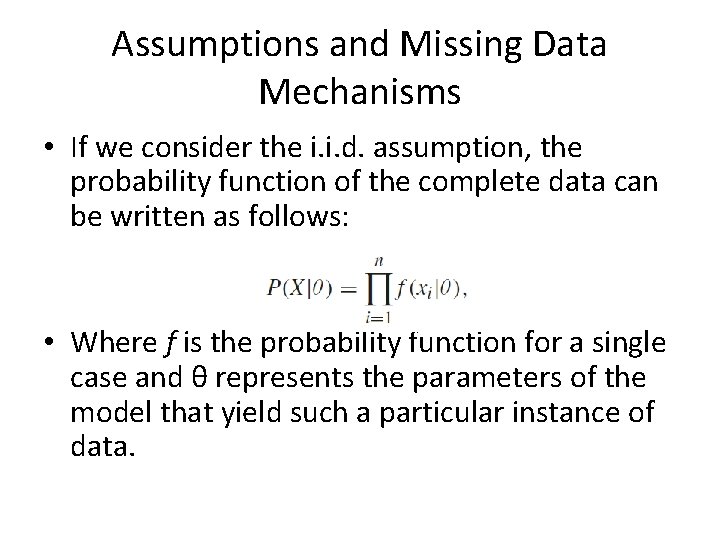
Assumptions and Missing Data Mechanisms • If we consider the i. i. d. assumption, the probability function of the complete data can be written as follows: • Where f is the probability function for a single case and θ represents the parameters of the model that yield such a particular instance of data.

Assumptions and Missing Data Mechanisms • The parameters’ values θ for the given data are very rarely known! • We can consider distributions that are commonly found in nature: – multivariate normal distribution (only real values) – multinomial model (nominal attributes) – mixed models for combined normal and categorical features

Assumptions and Missing Data Mechanisms • The parameters’ values θ for the given data are very rarely known! • We can consider distributions that are commonly found in nature: – multivariate normal distribution (only real values) – multinomial model (nominal attributes) – mixed models for combined normal and categorical features

Assumptions and Missing Data Mechanisms • X = (Xobs, Xmis), – We call Xobs the observed part of X – We denote the missing part as Xmis • Let’s suppose that we dispose of a matrix B of the same size of X • B values are 0 o 1 when X elements are missing and missing respectively.

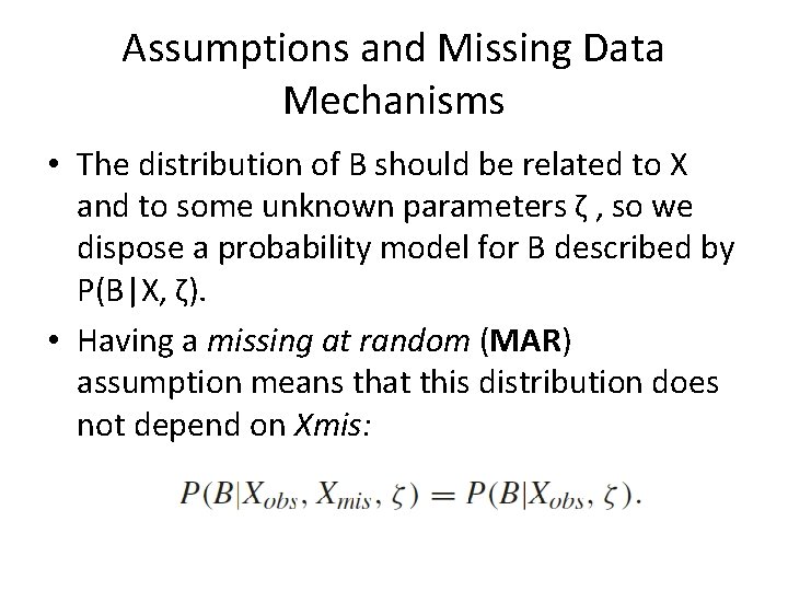
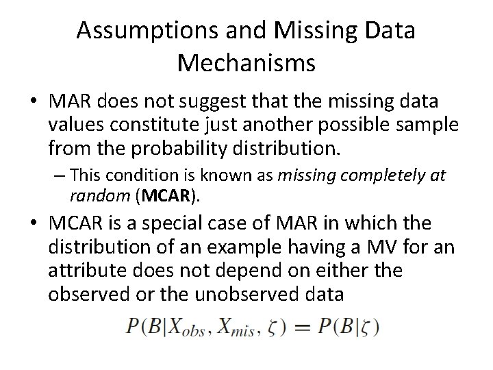
Assumptions and Missing Data Mechanisms • The distribution of B should be related to X and to some unknown parameters ζ , so we dispose a probability model for B described by P(B|X, ζ). • Having a missing at random (MAR) assumption means that this distribution does not depend on Xmis:

Assumptions and Missing Data Mechanisms • MAR does not suggest that the missing data values constitute just another possible sample from the probability distribution. – This condition is known as missing completely at random (MCAR). • MCAR is a special case of MAR in which the distribution of an example having a MV for an attribute does not depend on either the observed or the unobserved data

Assumptions and Missing Data Mechanisms • Under MCAR, the analysis of only those units with complete data gives valid inferences – Although there will generally be some loss of information • MCAR is more restrictive than MAR – MAR requires only that the MVs behave like a random sample of all values in some particular subclasses defined by observed data.

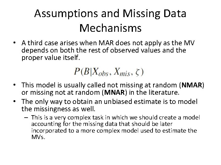
Assumptions and Missing Data Mechanisms • A third case arises when MAR does not apply as the MV depends on both the rest of observed values and the proper value itself. • This model is usually called not missing at random (NMAR) or missing not at random (MNAR) in the literature. • The only way to obtain an unbiased estimate is to model the missingness as well. – This is a very complex task in which we should create a model accounting for the missing data that should be later incorporated to a more complex model used to estimate the MVs.

Dealing with Missing Values 1. 2. 3. 4. 5. 6. Introduction Assumptions and Missing Data Mechanisms Simple Approaches to Missing Data Maximum Likelihood Imputation Methods Machine Learning Based Methods Experimental Comparative Analysis

Simple Approaches to Missing Data • They usually do not take into account the missingness mechanism and they blindly perform the operation.

Simple Approaches to Missing Data • The most simple approach is to do not impute (DNI). – the MVs remain unreplaced, so the DM algorithm must use their default MVs strategies if present • An alternative for these learning methods that cannot deal with MVs, another approach is to convert the MVs to a newvalue (encode them into a new numerical value). – Such a simplistic method has been shown to lead to serious inference problems

Simple Approaches to Missing Data • A very common approach in the specialized literature, even nowadays, is to apply case deletion or ignore missing (IM) – All instances with at least one MV are discarded from the data set. • Under the assumption that data is MCAR, it leads to unbiased parameter estimates… • … but even when the data are MCAR there is a loss in power using this approach

Simple Approaches to Missing Data • The substitution of the MVs for the global most common attribute value for nominal attributes, and global average value for numerical attributes (MC) is widely used • A variant of MC is the concept most common attribute value for nominal attributes, and concept average value for numerical attributes (CMC) – The MV is replaced by the most repeated one if nominal or is the mean value if numerical, but considers only the instances with the same class as the reference instance. • Drawback: the covariance in the imputed data set will be severely altered if the amount of MVs is considerable

Dealing with Missing Values 1. 2. 3. 4. 5. 6. Introduction Assumptions and Missing Data Mechanisms Simple Approaches to Missing Data Maximum Likelihood Imputation Methods Machine Learning Based Methods Experimental Comparative Analysis

Maximum Likelihood Imputation Methods • Rubin et al. formalized the concept of missing data introduction mechanisms and they advised against use case deletion as a methodology (IM) • An ideal and rare case would be where the parameters of the data distribution θ were known – A sample from such a distribution (conditioned or not to the other attributes’ values) would be a suitable imputed value for the missing one. • The problem is that the parameters θ are rarely known and also very hard to estimate

Maximum Likelihood Imputation Methods • An alternative is to use the maximum likelihood to estimate the original θ • So the next question arises: to solve a maximum likelihood type problem, can we analytically maximize the likelihood function? – it can work with one dimensional Bernoulli problems like the coin toss – it also works with onedimensional Gaussian by finding the μ and σ parameters

Maximum Likelihood Imputation Methods • Can we analytically maximize the likelihood function? • In real world data things are not that easy. – We can have distribution that may not be well behaved or – have too many parameters making the actual solution computationally too complex. • Having a likelihood function made of a mixture of 100 -dimensional Gaussians would yield 10, 000 parameters and thus direct trial-error maximization is not feasible.

Maximum Likelihood Imputation Methods • Can we analytically maximize the likelihood function? • In real world data things are not that easy. • The way to deal with such complexity is to introduce hidden variables in order to simplify the likelihood function and, in our case as well, to account for MVs. – The observed variables are those that can be directly measured from the data – hidden variables influence the data but are not trivial to measure • An example of an observed variable would be if it is sunny today, whereas the hidden variable can be P(sunny today|sunny yesterday).

Maximum Likelihood Imputation Methods • Even simplifying with hidden variables does not allow us to reach the solution in a single step. • The most common approach in these cases would be to use an iterative approach in which we obtain some parameter estimates, we use a regression technique to impute the values and repeat

Expectation-Maximization (EM) • In a nutshell the EM algorithm estimates the parameters of a probability distribution. • It iteratively maximizes the likelihood of the complete data Xobs considered as a function dependent of the parameters

Expectation-Maximization (EM) • That is, we want to model dependent random variables as the observed variable a and the hidden variable b that generates a • We stated that a set of unknown parameters θ governs the probability distributions Pθ (a), Pθ (b) • As an iterative process, the EM algorithm consists of two steps that are repeated until convergence: the expectation (E-step) and the maximization (M -step) steps.

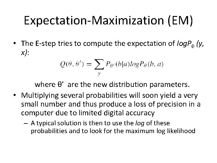
Expectation-Maximization (EM) • The E-step tries to compute the expectation of log. Pθ (y, x): where θ’ are the new distribution parameters. • Multiplying several probabilities will soon yield a very small number and thus produce a loss of precision in a computer due to limited digital accuracy – A typical solution is then to use the log of these probabilities and to look for the maximum log likelihood

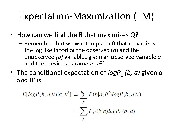
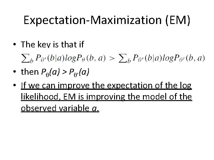
Expectation-Maximization (EM) • How can we find the θ that maximizes Q? – Remember that we want to pick a θ that maximizes the log likelihood of the observed (a) and the unobserved (b) variables given an observed variable a and the previous parameters θ’ • The conditional expectation of log. Pθ (b, a) given a and θ’ is

Expectation-Maximization (EM) • The key is that if • then Pθ(a) > Pθ’(a) • If we can improve the expectation of the log likelihood, EM is improving the model of the observed variable a.

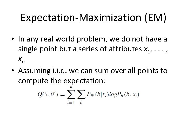
Expectation-Maximization (EM) • In any real world problem, we do not have a single point but a series of attributes x 1, . . . , xn • Assuming i. i. d. we can sum over all points to compute the expectation:

Expectation-Maximization (EM) • The EMalgorithm is not perfect: it can be stuck in local maxima and also depends on an initial θ value – The latter is usually resolved by using a bootstrap process in order to choose a correct initial θ • Also the reader may have noticed that we have not talked about any imputation yet. The reason is EM is a meta algorithm that it is adapted to a particular application

Expectation-Maximization (EM) • To use EM for imputation first we need to choose a plausible set of parameters – We need to assume that the data follows a probability distribution drawback • The EM algorithm works better with probability distributions that are easy to maximize Gaussian mixture models • In each iteration of the EM algorithm for imputation the estimates of the mean μ and the covariance Σ are represented by a matrix and revised in three phases • These parameters are used to apply a regression over the MVs by using the complete data.

Multiple Imputation (MI) • One big problem of the maximum likelihood methods like EM is that they tend to underestimate the inherent errors produced by the estimation process, formally standard errors. • The Multiple Imputation (MI) approach was designed to take this into account to be a less biased imputation method, at the cost of being computationally expensive.

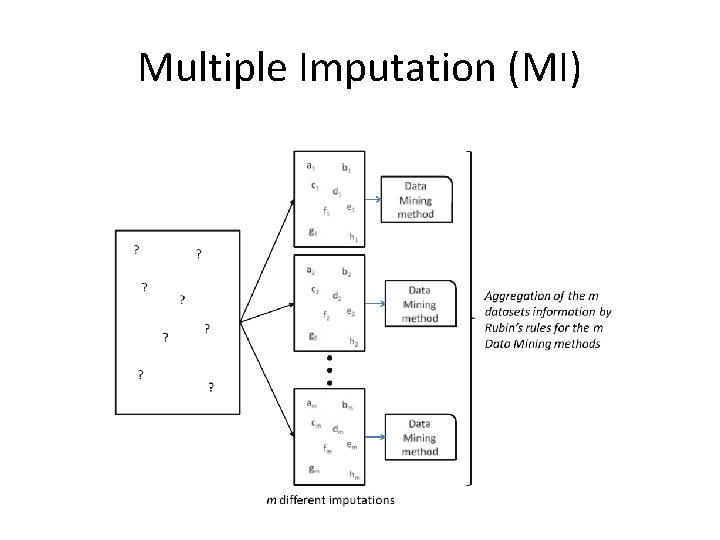
Multiple Imputation (MI) • MI is a Monte Carlo approach in which we generate multiple imputed values from the observed data in a very similar way to the EM algorithm – it fills the incomplete data by repeatedly solving the observed data • But a significative difference between the two methods is attained: – EM generates a single imputation in each step from the estimated parameters at each step, – MI performs several imputations that yield several complete data sets Data Augmentation (DA)

Multiple Imputation (MI)

Multiple Imputation (MI) • This repeated imputation can be done thanks to the use of Markov Chain Monte Carlo methods • Several imputations are obtained by introducing a random component, usually from a standard normal distribution

Multiple Imputation (MI) • In a more advanced fashion, MI also considers that the parameters estimates are in fact sample estimates • The parameters are not directly estimated from the available data but, as the process continues, they are drawn from their Bayesian posterior distributions given the data at hand – These assumptions means that only in the case of MCAR or MAR missingness mechanisms hold MI should be applied.

Multiple Imputation (MI) • Due to its Bayesian nature, the user needs to specify a prior distribution for the parameters θ of the model • In practice is stressed out that the results depend more on the election of the distribution for the data than the distribution for θ

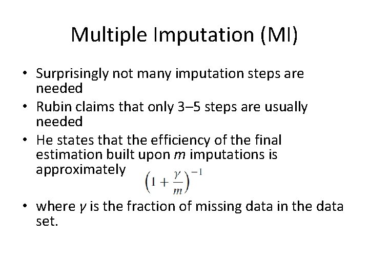
Multiple Imputation (MI) • Surprisingly not many imputation steps are needed • Rubin claims that only 3– 5 steps are usually needed • He states that the efficiency of the final estimation built upon m imputations is approximately • where γ is the fraction of missing data in the data set.

Multiple Imputation (MI) • With a 30% of MVs in each data set, which is a quite high amount, with 5 different final data sets a 94% of efficiency will be achieved • Increasing the number to m = 10 slightly raises the efficiency to 97%, which is a low gain paying the double computational effort.

Multiple Imputation (MI) • With a 30% of MVs in each data set, which is a quite high amount, with 5 different final data sets a 94% of efficiency will be achieved • Increasing the number to m = 10 slightly raises the efficiency to 97%, which is a low gain paying the double computational effort.

Multiple Imputation (MI) • To start we need an estimation of the mean and covariance matrices. – A good approach is to take them from a solution provided from an EM algorithm once their values have stabilized at the end of its execution • Then the DA process starts by alternately filling the MVs and then making inferences about the unknown parameters in a stochastic fashion: 1. 2. DA creates an imputation using the available values of the parameters of the MVs Draws new parameter values from the Bayesian posterior distribution using the observed and missing data • Concatenating this process of simulating the MVs and the parameters is what creates a Markov chain that will converge at some point

Multiple Imputation (MI) • The iterative process will converge: – The distribution of the parameters θ will stabilize to the posterior distribution averaged over the MVs – The distribution of the MVs will stabilize to a predictive distribution: the proper distribution needed to drawn values for the MIs. • Large rates of MVs in the data sets will cause the convergence to be slow

Multiple Imputation (MI) • However, the meaning of convergence is different to that used in EM – In EM the parameter estimates have converged when they no longer change from one iteration to the following over a threshold – In DA the distribution of the parameters do not change across iterations but the random parameter values actually continue changing, which makes the convergence of DA more difficult to assess than for EM

Multiple Imputation (MI) • Convergence is reinterpreted in MI: – DA can be said to have converged by k cycles if the value of any parameter at iteration t ∈ 1, 2, . . . is statistically independent of its value at iteration t +k • The DA algorithm usually converges under these terms in equal or less cycles than EM.

Multiple Imputation (MI) • The value k is interesting: – it establishes when we should stop performing the Markov chain in order to have MI that are independent draws from the missing data predictive distribution. • A typical process is to perform m runs, each one of length k – for each imputation from 1 to m we perform the DA process during k cycles • It is a good idea not to be too conservative with the k value, as after convergence the process remains stationary, whereas with low k values the m imputed data sets will not be truly independent. – Remember that we do not need a high m value, so k acts as the true computational effort measure.

Multiple Imputation (MI) • Once the m MI data sets have been created, they can be analyzed by any standard complete-data methods • For example, we can use a linear or logistic regression, a classifier or any other technique applied to each one of the m data sets • The variability of the m results obtained will reflect the uncertainty of MVs

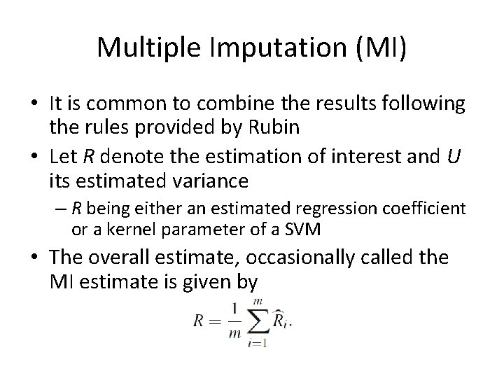
Multiple Imputation (MI) • It is common to combine the results following the rules provided by Rubin • Let R denote the estimation of interest and U its estimated variance – R being either an estimated regression coefficient or a kernel parameter of a SVM • The overall estimate, occasionally called the MI estimate is given by

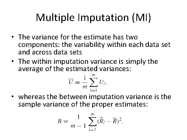
Multiple Imputation (MI) • The variance for the estimate has two components: the variability within each data set and across data sets • The within imputation variance is simply the average of the estimated variances: • whereas the between imputation variance is the sample variance of the proper estimates:

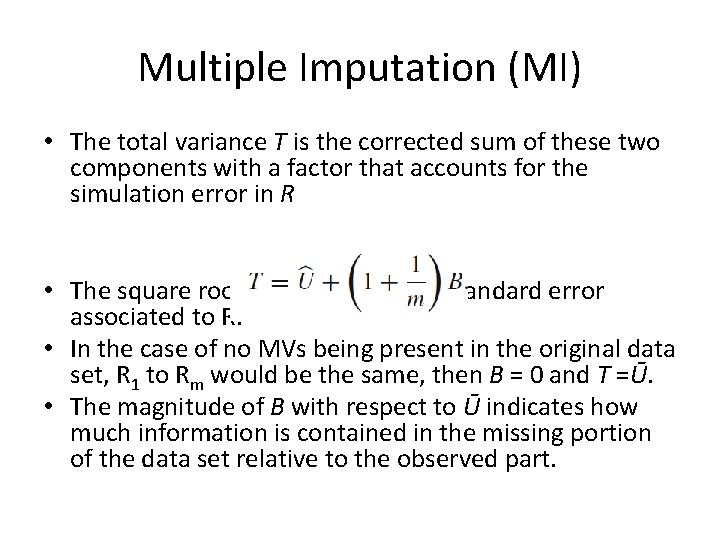
Multiple Imputation (MI) • The total variance T is the corrected sum of these two components with a factor that accounts for the simulation error in R • The square root of T is the overall standard error associated to R. • In the case of no MVs being present in the original data set, R 1 to Rm would be the same, then B = 0 and T =Ū. • The magnitude of B with respect to Ū indicates how much information is contained in the missing portion of the data set relative to the observed part.

Bayesian Principal Component Analysis (BPCA) • The MV estimation method based on BPCA consists of three elementary processes: 1. Principal component (PC) regression 2. Bayesian estimation 3. An EM-like repetitive algorithm

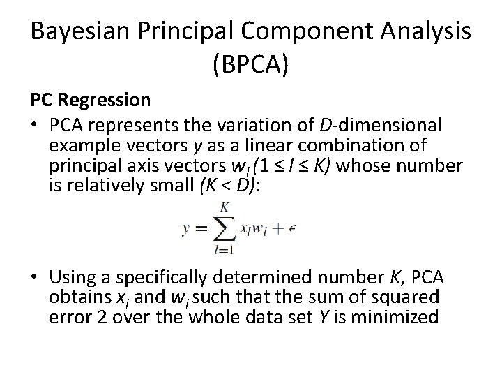
Bayesian Principal Component Analysis (BPCA) PC Regression • PCA represents the variation of D-dimensional example vectors y as a linear combination of principal axis vectors wl (1 ≤ l ≤ K) whose number is relatively small (K < D): • Using a specifically determined number K, PCA obtains xl and wl such that the sum of squared error 2 over the whole data set Y is minimized

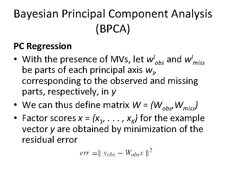
Bayesian Principal Component Analysis (BPCA) PC Regression • With the presence of MVs, let wlobs and wlmiss be parts of each principal axis wl, corresponding to the observed and missing parts, respectively, in y • We can thus define matrix W = (Wobs, Wmiss) • Factor scores x = (x 1, . . . , x. K) for the example vector y are obtained by minimization of the residual error

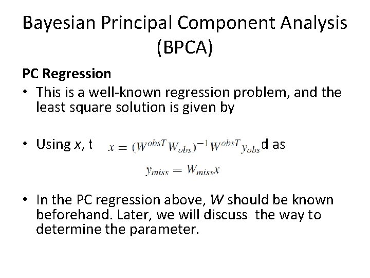
Bayesian Principal Component Analysis (BPCA) PC Regression • This is a well-known regression problem, and the least square solution is given by • Using x, the missing part is estimated as • In the PC regression above, W should be known beforehand. Later, we will discuss the way to determine the parameter.

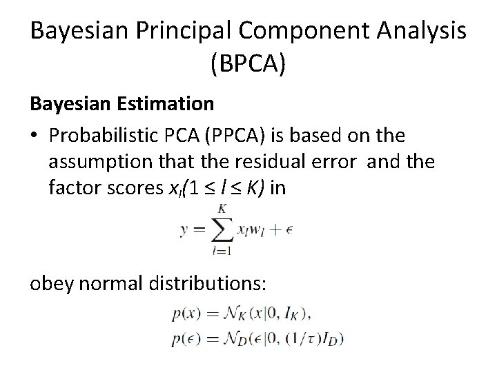
Bayesian Principal Component Analysis (BPCA) Bayesian Estimation • Probabilistic PCA (PPCA) is based on the assumption that the residual error and the factor scores xl(1 ≤ l ≤ K) in obey normal distributions:

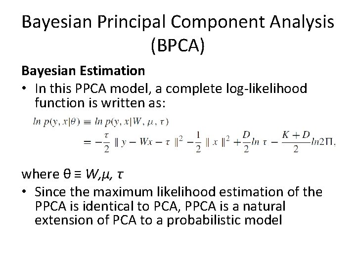
Bayesian Principal Component Analysis (BPCA) Bayesian Estimation • In this PPCA model, a complete log-likelihood function is written as: where θ ≡ W, μ, τ • Since the maximum likelihood estimation of the PPCA is identical to PCA, PPCA is a natural extension of PCA to a probabilistic model

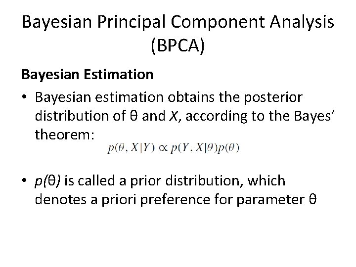
Bayesian Principal Component Analysis (BPCA) Bayesian Estimation • Bayesian estimation obtains the posterior distribution of θ and X, according to the Bayes’ theorem: • p(θ) is called a prior distribution, which denotes a priori preference for parameter θ

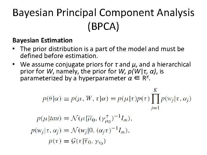
Bayesian Principal Component Analysis (BPCA) Bayesian Estimation • The prior distribution is a part of the model and must be defined before estimation. • We assume conjugate priors for τ and μ, and a hierarchical prior for W, namely, the prior for W, p(W|τ, α), is parameterized by a hyperparameter α ∈ RK.

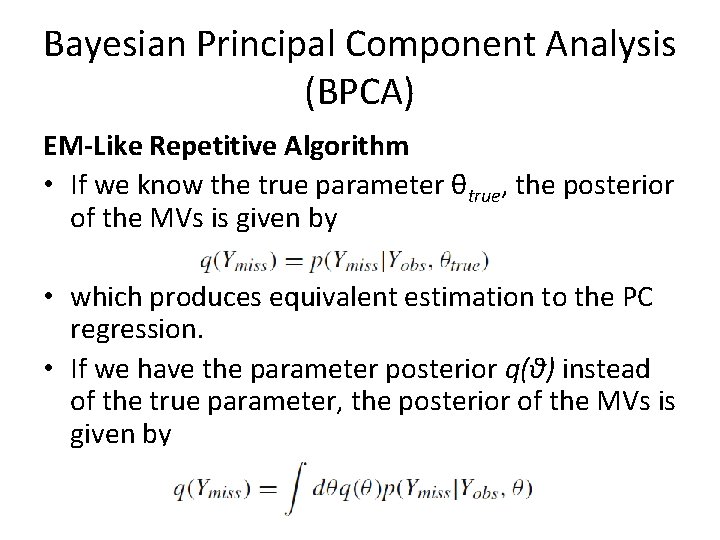
Bayesian Principal Component Analysis (BPCA) EM-Like Repetitive Algorithm • If we know the true parameter θtrue, the posterior of the MVs is given by • which produces equivalent estimation to the PC regression. • If we have the parameter posterior q(θ) instead of the true parameter, the posterior of the MVs is given by

Bayesian Principal Component Analysis (BPCA) EM-Like Repetitive Algorithm • Since we do not know the true parameter naturally, we conduct the BPCA • The parameter posterior q(θ) with MVs requires to obtain q(θ) and q(Ymiss) simultaneously • We can use a variational Bayes (VB) algorithm, in order to execute Bayesian estimation for both model parameter θ and MVs Ymiss.

Bayesian Principal Component Analysis (BPCA) EM-Like Repetitive Algorithm • The VB algorithm resembles the EM algorithm: – It obtains maximum likelihood estimators for θ and Ymiss, but… – …it obtains the posterior distributions for θ and Ymiss, q(θ) and q(Ymiss), by a repetitive algorithm.

Bayesian Principal Component Analysis (BPCA) EM-Like Repetitive Algorithm • The VB algorithm is implemented as follows: 1. the posterior distribution of MVs, q(Ymiss), is initialized by imputing each of the MVs to instance-wise average; 2. the posterior distribution of the parameter θ, q(θ), is estimated using the observed data Yobs and the current posterior distribution of MVs, q(Ymiss); 3. the posterior distribution of the MVs, q(Ymiss), is estimated using the current q(θ); 4. the hyperparameter α is updated using both of the current q(θ) and the current q(Ymiss); 5. repeat 2– 4 until convergence.

Dealing with Missing Values 1. 2. 3. 4. 5. 6. Introduction Assumptions and Missing Data Mechanisms Simple Approaches to Missing Data Maximum Likelihood Imputation Methods Machine Learning Based Methods Experimental Comparative Analysis

Machine Learning Based Methods • The imputation methods presented in previous section originated from statistics application – they model the relationship between the values by searching for the hidden distribution probabilities. • In Artificial Intelligence modeling the unknown relationships between attributes and the inference of the implicit information contained in a sample data set has been done using Machine Learning models.

Machine Learning Based Methods • The same process used to predict a continuous or a nominal value from a previous learning process in regression or classification can be applied to predict the MVs. • The use of ML methods for imputation alleviates us from searching for the estimated underlying distribution of the data – but they are still subject to the MAR assumption in order to correctly apply them

Imputation with K-Nearest Neighbor (KNNI) • Using this instance-based algorithm, every time a MV is found in a current instance, KNNI computes the KNN and a value from them is imputed – For nominal values, the most common value among all neighbors is taken – For numerical values the average value is used • A proximity measure between instances is needed for it to be defined. – The Euclidean distance (it is a case of a Lp norm distance) is the most commonly used in the literature.

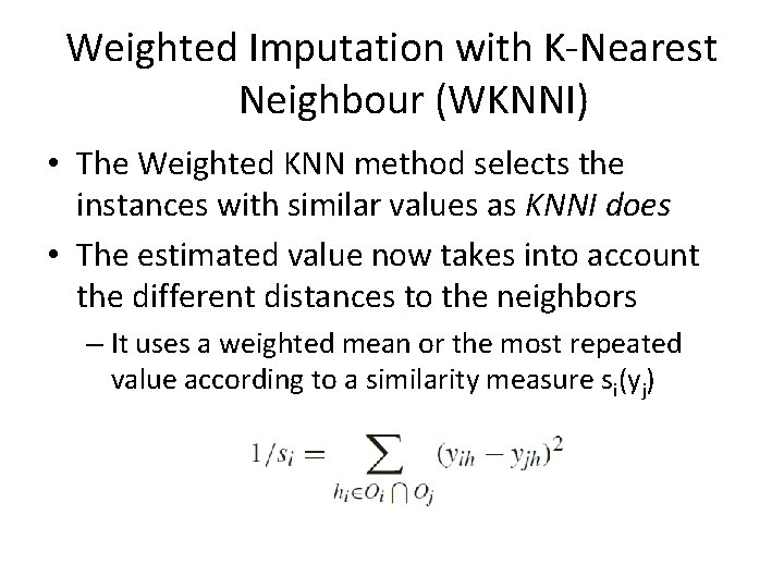
Weighted Imputation with K-Nearest Neighbour (WKNNI) • The Weighted KNN method selects the instances with similar values as KNNI does • The estimated value now takes into account the different distances to the neighbors – It uses a weighted mean or the most repeated value according to a similarity measure si(yj)

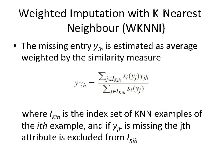
Weighted Imputation with K-Nearest Neighbour (WKNNI) • The missing entry yih is estimated as average weighted by the similarity measure where IKih is the index set of KNN examples of the ith example, and if yjh is missing the jth attribute is excluded from IKih

K-means Clustering Imputation (KMI) • In K-means clustering the overall objective is to divide the data set into groups based on the similarity of objects • A cluster centroid represents the mean value of the objects in the cluster • K-means measures the intra-cluster dissimilarity by the addition of distances among the objects and the centroid of the cluster

K-means Clustering Imputation (KMI) • In KMI, once the clusters have converged, the last process is to fill in all the non-reference attributes for each incomplete object based on the cluster information • Data objects that belong to the same cluster are taken to be nearest neighbors of each other, and KMI applies a nearest neighbor algorithm to replace MVs, in a similar way to KNNI

Fuzzy K-means Clustering (FKMI) • In fuzzy clustering, each data object has a membership function U which describes the degree to which this data object belongs to a certain cluster • The original K-means clustering may be trapped in a local minimum status if the initial points are not selected properly – Continuous membership values in fuzzy clustering make the resulting algorithms less susceptible to get stuck in a local minimum situation

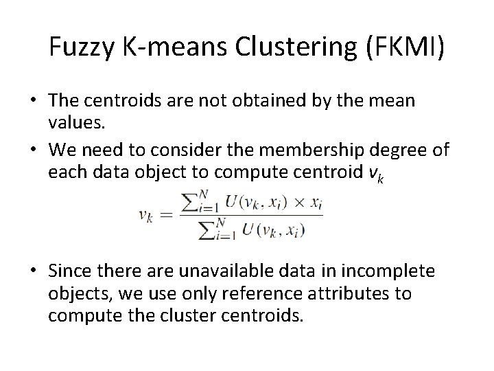
Fuzzy K-means Clustering (FKMI) • The centroids are not obtained by the mean values. • We need to consider the membership degree of each data object to compute centroid vk • Since there are unavailable data in incomplete objects, we use only reference attributes to compute the cluster centroids.

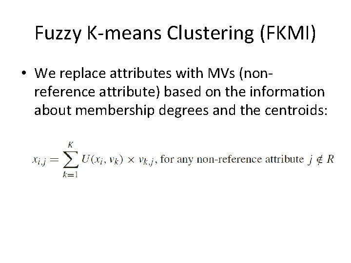
Fuzzy K-means Clustering (FKMI) • We replace attributes with MVs (nonreference attribute) based on the information about membership degrees and the centroids:

Support Vector Machines Imputation (SVMI) • Support Vector Machines Imputation is an SVM regression based algorithm to fill in MVs – If the attribute with MVs is nominal it will act as a SVM classifier • It sets the decision attributes (output or classes) as the condition attributes (input attributes) and the condition attributes as the decision attributes – Only the instances without MVs are used to predict the MV currently being imputed

Event Covering (EC) • In EC mixed-mode probability model is approximated by a discrete one – We discretize the continuous components using a minimum loss of information criterion • Treating a mixed-mode feature n-tuple as a discrete-valued one, the authors propose a new statistical approach for synthesis of knowledge based on cluster analysis

Event Covering (EC) • EC consists of 3 steps: 1. detect from data patterns which indicate statistical interdependency 2. group the given data into clusters based ondetected interdependency 3. interpret the underlying patterns for each of the clusters identified

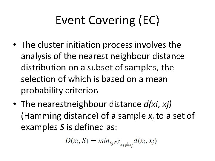
Event Covering (EC) • The cluster initiation process involves the analysis of the nearest neighbour distance distribution on a subset of samples, the selection of which is based on a mean probability criterion • The nearestneighbour distance d(xi, xj) (Hamming distance) of a sample xi to a set of examples S is defined as:

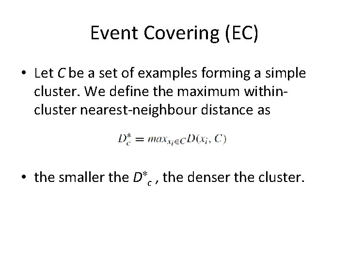
Event Covering (EC) • Let C be a set of examples forming a simple cluster. We define the maximum withincluster nearest-neighbour distance as • the smaller the D∗c , the denser the cluster.

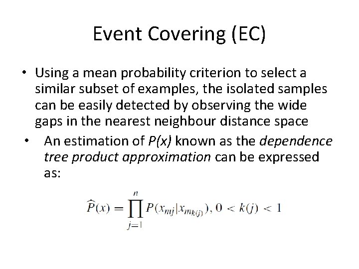
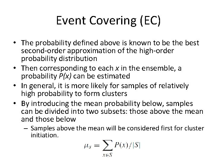
Event Covering (EC) • Using a mean probability criterion to select a similar subset of examples, the isolated samples can be easily detected by observing the wide gaps in the nearest neighbour distance space • An estimation of P(x) known as the dependence tree product approximation can be expressed as:

Event Covering (EC) • The probability defined above is known to be the best second-order approximation of the high-order probability distribution • Then corresponding to each x in the ensemble, a probability P(x) can be estimated • In general, it is more likely for samples of relatively high probability to form clusters • By introducing the mean probability below, samples can be divided into two subsets: those above the mean and those below – Samples above the mean will be considered first for cluster initiation.

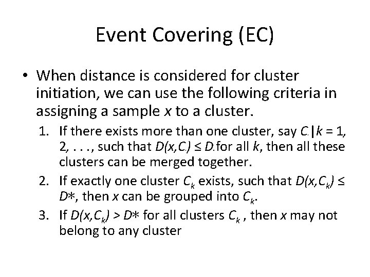
Event Covering (EC) • When distance is considered for cluster initiation, we can use the following criteria in assigning a sample x to a cluster. 1. If there exists more than one cluster, say C |k = 1, 2, . . . , such that D(x, C ) ≤ D for all k, then all these clusters can be merged together. 2. If exactly one cluster Ck exists, such that D(x, Ck) ≤ D∗, then x can be grouped into Ck. 3. If D(x, Ck) > D∗ for all clusters Ck , then x may not belong to any cluster k k ∗

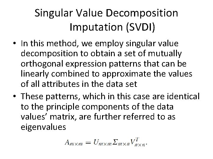
Singular Value Decomposition Imputation (SVDI) • In this method, we employ singular value decomposition to obtain a set of mutually orthogonal expression patterns that can be linearly combined to approximate the values of all attributes in the data set • These patterns, which in this case are identical to the principle components of the data values’ matrix, are further referred to as eigenvalues

Singular Value Decomposition Imputation (SVDI) • Matrix VT now contains eigenvalues, whose contribution to the expression in the eigenspace is quantified by corresponding eigenvalues on the diagonal of matrix Σ • We then identify the most significant eigenvalues by sorting the eigenvalues based on their corresponding eigenvalue – the exact fraction of eigenvalues best for estimation needs to be determined empirically

Singular Value Decomposition Imputation (SVDI) • Once k most significant eigenvalues from VT are selected, we estimate a MV j in example i by first regressing this attribute value against the k eigenvalues and then use the coefficients of the regression to reconstruct j from a linear combination of the k eigenvalues – The jth value of example i and the jth values of the k eigenvalues are not used in determining these regression coefficients

Singular Value Decomposition Imputation (SVDI) • It should be noted that SVD can only be performed on complete matrices • A good approximation is to first apply EM to complete the matrix in order to obtain the eigenvectors and eigenvalues

Local Least Squares Imputation (LLSI) • In this method a target instance that has MVs is represented as a linear combination of similar instances • Rather than using all available instances in the data, only similar instances based on a similarity measure are used

Local Least Squares Imputation (LLSI) • There are two steps in the LLSI 1. To select k instances by the L 2 -norm 2. Regression and estimation, regardless of how the k instances are selected • A heuristic k parameter selection method is used by the authors based on Pearson’s correlation coefficient

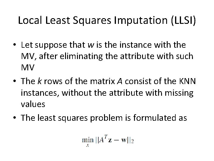
Local Least Squares Imputation (LLSI) • Let suppose that w is the instance with the MV, after eliminating the attribute with such MV • The k rows of the matrix A consist of the KNN instances, without the attribute with missing values • The least squares problem is formulated as

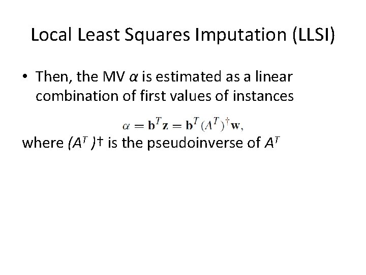
Local Least Squares Imputation (LLSI) • Then, the MV α is estimated as a linear combination of first values of instances where (AT )† is the pseudoinverse of AT

Recent Machine Learning Approaches • There is a great amount of journal publications showing their application and particularization to real world problems • They can be grouped by the paradigm in which they are based on: – Clustering: MLP hybrid, LLS based, Fuzzy c-means with SVR and GAs, Hierarchical Clustering, K 2 clustering, Weighted K-means, etc. – ANNs: RBFN based, Wavelet ANNs, MLP, ANNs framework, SOM, – Bayesian networks: Dynamic bayesian networks, Bayesian networks with weights, Mixture-kernel-based iterative estimator – Nearest neighbors: ICk. NNI, Iterative KNNI, CGImpute, Boostrap for maximum likelihood, k. DMI – Ensembles: Random Forest, Decision forest, GMDH – Similarity and correlation: FIMUS – Parameter estimation for regression imputation: EAs for covariance matrix estimation, Iterative mutual information imputation, CMVE, DMI (EM + decision trees), WLLSI

Dealing with Missing Values 1. 2. 3. 4. 5. 6. Introduction Assumptions and Missing Data Mechanisms Simple Approaches to Missing Data Maximum Likelihood Imputation Methods Machine Learning Based Methods Experimental Comparative Analysis

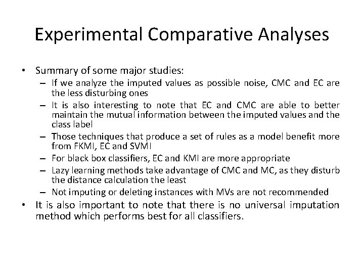
Experimental Comparative Analyses • Summary of some major studies: – If we analyze the imputed values as possible noise, CMC and EC are the less disturbing ones – It is also interesting to note that EC and CMC are able to better maintain the mutual information between the imputed values and the class label – Those techniques that produce a set of rules as a model benefit more from FKMI, EC and SVMI – For black box classifiers, EC and KMI are more appropriate – Lazy learning methods take advantage of CMC and MC, as they disturb the distance calculation the least – Not imputing or deleting instances with MVs are not recommended • It is also important to note that there is no universal imputation method which performs best for all classifiers.