MISSING DATA AND DROPOUT What is missing data

MISSING DATA AND DROPOUT

What is missing data? • Missing data arise in longitudinal studies whenever one or more of the sequences of measurements are incomplete, in the sense that some intended measurements are not obtained.

Missing data • Let Y denote the complete response vector which can be partitioned into two sub-vectors: (i) (ii) the measurements observed the measurements that are missing

Missing data • If there were no missing data, we would have observed the complete response vector Y. • Instead, we get to observe .

What is the problem? • The main problem that arises with missing data is that the distribution of the observed data may not be the same as the distribution of the complete data.

Consider the following simple illustration: • Suppose we intend to measure subjects at 6 months (Y 1) and 12 months (Y 2) post treatment. • All of the subjects return for measurement at 6 months, but many do not return at 12 months.

• If subjects fail to return for measurement at 12 months because they are not well (say, values of Y 2 are low), then the distribution of observed Y 2’s will be positively skewed compared to the distribution of Y 2’s in the population of interest.

• In general, the situation may often be quite complex, with some missingness unrelated to either the observed or unobserved response, some related to the observed, some related to the unobserved, and some to both.

Monotone missing data • A particular pattern of missingness that is common in longitudinal studies is ‘dropout’ or ‘attrition’. This is where an individual is observed from baseline up until a certain point in time, thereafter no more measurements are made.

Study Dropout Possible reasons for dropout: 1. 2. 3. 4. 5. Recovery Lack of improvement or failure Undesirable side effects External reasons unrelated to specific treatment or outcome Death

Examples • In clinical trials, missing data can arise from a variety of circumstances: a) Late entrants: If the study has staggered entry, at any interim analysis some individuals may have only partial response data. Usually, this sort of missing data does not introduce any bias.

b) Dropout: Individuals may drop out of a clinical trial because of side effects or lack of efficacy. Usually, this type of missing data is of concern, especially if dropout is due to lack of efficacy. Dropout due to lack of efficacy suggests that those who drop out come from the lower end of the spectrum. Dropout due to side effects may or may not be a problem, depending upon the relationship between side effects and the outcome of interest.

Intermittent vs Dropout Missing Data • important feature is whether the missing values pattern is dropout (monotone) or intermittent (nonmonotone). • The dropout pattern, in the sense that some subjects may withdraw prematurely, i. e. any missing value is never followed by an observed value. • The intermittent pattern whenever an observed value is available even after a missing value occurs.

• Examples of intermittent missing data?

Type of missing data • A hierarchy of three different types of missing data mechanisms can be distinguished: 1) Data are missing completely at random (MCAR) when the probability that an individual value will be missing is independent of Y(o) and Y(m).

2) 3) Data are missing at random (MAR) when the probability that an individual value will be missing is independent of Y(m) (but may depend on Y(o)). Missing data are nonignorable when the probability that an individual value will be missing depends on Y(m).

• Note: Under assumptions 1) and 2), the missing data mechanism is often referred to as being ‘ignorable’. • If missingness depends only on X, then technically it is MCAR. However, sometimes this is referred to as covariate dependent non-response.

• Thus, in general, if non-response depends on covariates, X, it is harmless and the same as MCAR provided you always condition on the covariates (i. e. , incorporate the covariate in the analysis). This type of missingness is only a problem if you do not condition on X.

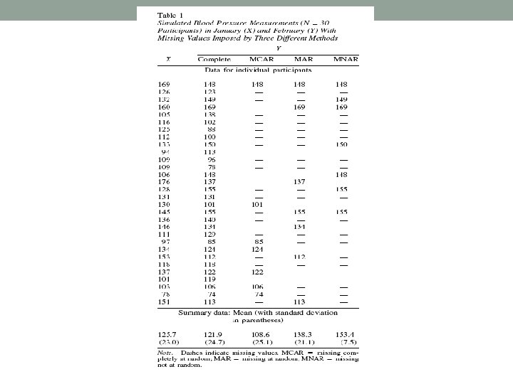
Example • Suppose that systolic blood pressures of N participants are recorded in January (X). Some of them have a second reading in February (Y), but others do not. Table 1 shows simulated data for N = 30 participants drawn from a bivariate normal population with means mx =my = 125, standard deviations sx = sy = 25, and correlation r=0. 60.

• The first two columns of the measurements exceeded 140 (X > 140), a level used for diagnosing hypertension; this is MAR but not MCAR. In the third method, those recorded in February were those whose February measurements exceeded 140 (Y > 140).

• This could happen, for example, if all individuals returned in February, but the staff person in charge decided to record the February value only if it was in the hypertensive range. This third mechanism is an example of MNAR. (Other MNAR mechanisms are possible; e. g. , the February measurement may be recorded only if it is substantially different from the January reading. )

• Notice that as we move from MCAR to MNAR, the observed Y values become an increasingly select and unusual group relative to the population; the sample mean increases, and the standard deviation decreases. This phenomenon is not a universal feature of MCAR, MAR, and MNAR, but it does happen in many realistic examples.

Methods of Handling Missing Data 1. Complete Case Methods: These methods omit all cases with missing values at any measurement occasion. Drawbacks: i. Can results in a very substantial loss of information which has an impact on precision and power. ii. Can give severely biased results if complete cases are not a random sample of population of interest, i. e. complete case methods require MCAR assumption.

2. All Available Case Methods: This is a general term for a variety of different methods that use the available information to estimate means and covariances (the latter based on all available pairs of cases). • In general, these methods are more efficient than complete case methods (and can be fully efficient in some cases).

Drawbacks: i. Sample base of cases changes over measurement occasions. ii. Available case methods require MCAR assumption (sometimes MAR).

3. Single Imputation Methods: These are methods that fill in the missing values. Once imputation is done, the analysis is straightforward.

Drawbacks: i. Systematically underestimate the variance and covariance. Treating imputed data as real data leads to standard errors that are too small (multiple imputation addresses this problem). ii. Produce biased estimates under any kind of missingness.

• Last Value Carried Forward: Set the response equal to the last observed value (or sometimes the ‘worst’ observed value). • In general, LVCF is not recommended!

4. Likelihood-based Methods: At least in • principle, maximum likelihood estimation for incomplete data is the same as for complete data and provides valid estimates and standard errors for more general circumstances than methods 1), 2), or 3). That is, under clearly stated assumptions likelihood-based methods have optimal statistical properties.

• For example, if missing data are ‘ignorable’ (MCAR/MAR), likelihood-based methods (e. g. PROC MIXED) simply maximize the marginal distribution of the observed responses. • If missing data are ‘non-ignorable’, likelihoodbased inference must also explicitly (and correctly) model the non-response process. However, with ‘non-ignorable’ missingness the methods are very sensitive to unverifiable assumptions.

5. • Weighting Methods: Base estimation on observed data, but weight the data to account for missing data. Basic idea: some sub-groups of the population are under-represented in the observed data, therefore weight these up to compensate for underrepresentation.

• For example, with dropout, can estimate the weights as a function of the individual’s covariates and responses up until the time of dropout. • This approach is valid provided the model for dropout is correct, i. e. provided the correct weights are available.

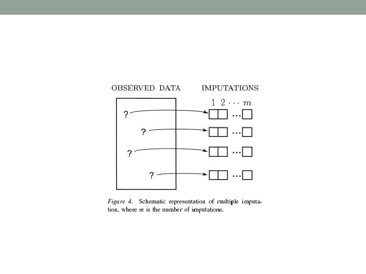
6. Multiple imputation: Each missing value is replaced by a list of m>1 simulated values. Each of the m data sets is analyzed in the same fashion by a complete-data method. The results are then combined by simple arithmetic to obtain overall estimates and stand errors that reflects missing data uncertainty as well as finite sample variation.

• The simplest method for combining the results of m analyses is Rubin’s (1987) method for a scalar (onedimensional) parameter. Suppose that Q represents a population quantity (e. g. , a regression coefficient) to be estimated. Let Q* and U* denote the estimate of Q and the standard error that one would use if no data were missing.

• The method assumes that the sample is large enough so that sqrt(U*)(Q * − Q) has approximately a standard normal distribution, so that Q * ± 1. 96 sqrt( U*) has about 95% coverage.

• Of course, we cannot compute Q* and U*; rather, we have m different versions of them, [Q* ( j), U*( j)], j _=1, . . . , m. Rubin’s (1987) overall estimate is simply the average of the m estimates,

• The uncertainy in Q has two parts: the average within imputation variance, and the between-imputations variance,

• The total variance is a modified sum of the two components, and the square root of T is the overall standard error.