Data Analytics CS 40003 Lecture 7 Relation Analysis

Data Analytics (CS 40003) Lecture #7 Relation Analysis Dr. Debasis Samanta Associate Professor Department of Computer Science & Engineering

Quote of the day. . Nothing great was ever achieved without enthusiasm. � RALPH WALDO EMERSON, American philosopher CS 40003: Data Analytics 2

This presentation includes… � CS 40003: Data Analytics 3

Hypothesis Testing Strategies � There are two types of tests of hypotheses üParametric tests (also called standard test of hypotheses). q Non-parametric tests (also called distribution-free test of hypotheses) CS 40003: Data Analytics 4

Parametric Tests : Applications � Usually assume certain properties of the population from which we draw samples. • Observation come from a normal population • Sample size is small • Population parameters like mean, variance, etc. are hold good. • Requires measurement equivalent to interval scaled data. CS 40003: Data Analytics 5

Hypothesis Testing : Non-Parametric Test �Non-Parametric tests o Does not under any assumption o Assumes only nominal or ordinal data Note: Non-parametric tests need entire population (or very large sample size) CS 40003: Data Analytics 6

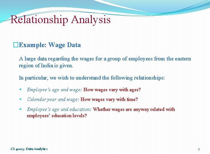
Relationship Analysis �Example: Wage Data A large data regarding the wages for a group of employees from the eastern region of India is given. In particular, we wish to understand the following relationships: § Employee’s age and wage: How wages vary with ages? § Calendar year and wage: How wages vary with time? § Employee’s age and education: Whether wages are anyway related with employees’ education levels? CS 40003: Data Analytics 7

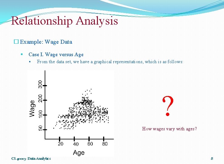
Relationship Analysis � Example: Wage Data § Case I. Wage versus Age § From the data set, we have a graphical representations, which is as follows: ? § How wages vary with ages? CS 40003: Data Analytics How wages vary with ages? 8

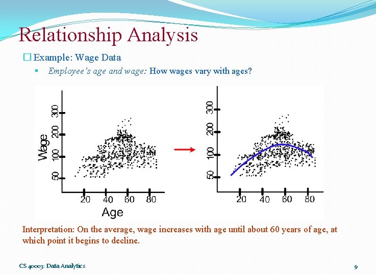
Relationship Analysis � Example: Wage Data § Employee’s age and wage: How wages vary with ages? Interpretation: On the average, wage increases with age until about 60 years of age, at which point it begins to decline. CS 40003: Data Analytics 9

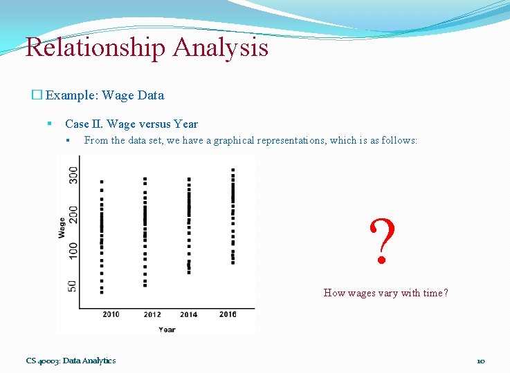
Relationship Analysis � Example: Wage Data § Case II. Wage versus Year § From the data set, we have a graphical representations, which is as follows: ? How wages vary with time? CS 40003: Data Analytics 10

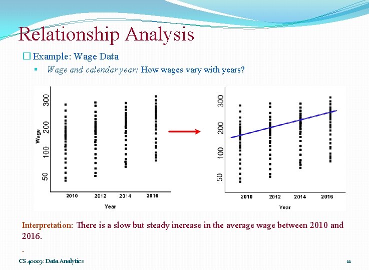
Relationship Analysis � Example: Wage Data § Wage and calendar year: How wages vary with years? Interpretation: There is a slow but steady increase in the average wage between 2010 and 2016. . CS 40003: Data Analytics 11

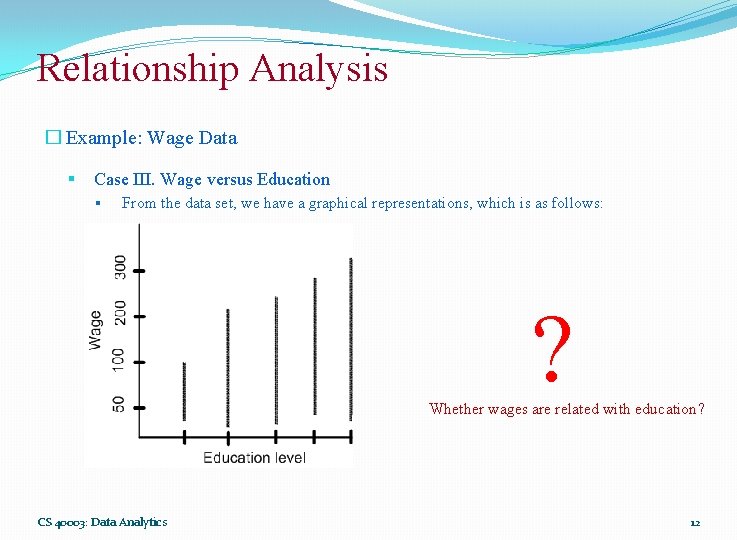
Relationship Analysis � Example: Wage Data § Case III. Wage versus Education § From the data set, we have a graphical representations, which is as follows: ? Whether wages are related with education? CS 40003: Data Analytics 12

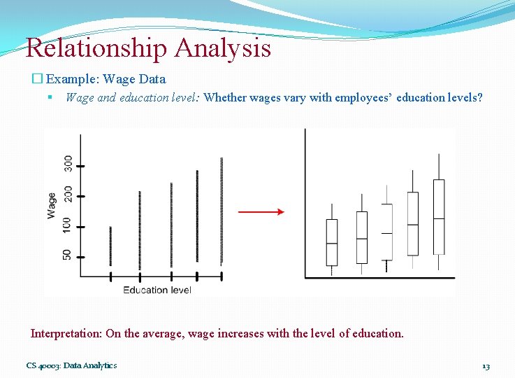
Relationship Analysis � Example: Wage Data § Wage and education level: Whether wages vary with employees’ education levels? Interpretation: On the average, wage increases with the level of education. CS 40003: Data Analytics 13

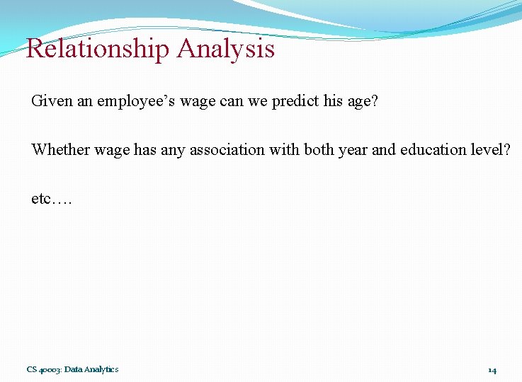
Relationship Analysis Given an employee’s wage can we predict his age? Whether wage has any association with both year and education level? etc…. CS 40003: Data Analytics 14

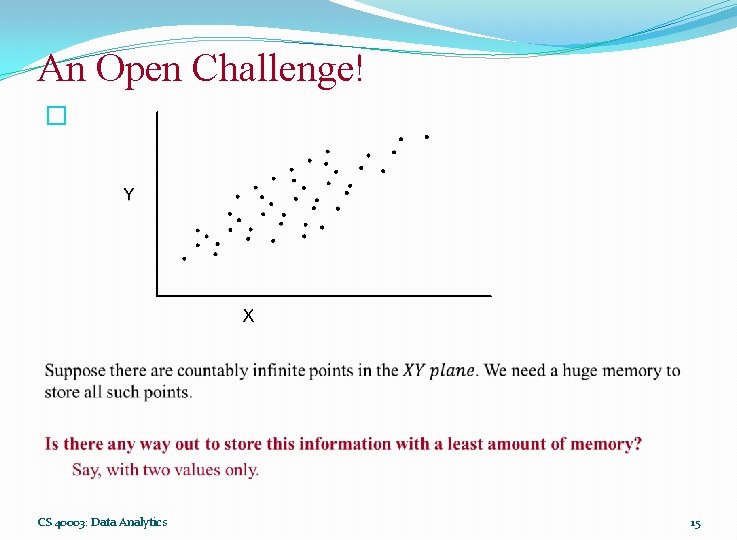
An Open Challenge! � CS 40003: Data Analytics 15

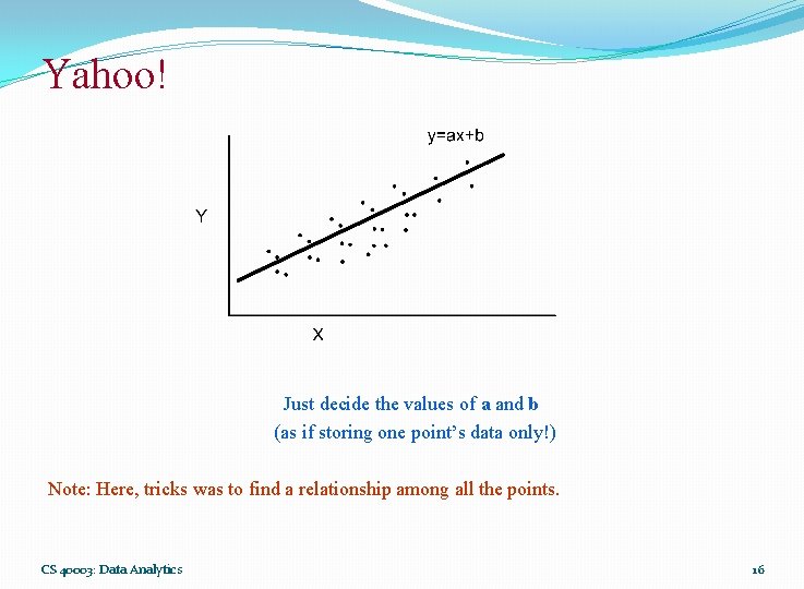
Yahoo! Just decide the values of a and b (as if storing one point’s data only!) Note: Here, tricks was to find a relationship among all the points. CS 40003: Data Analytics 16

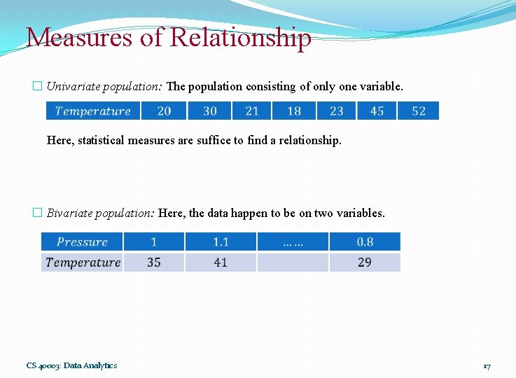
Measures of Relationship � Univariate population: The population consisting of only one variable. Here, statistical measures are suffice to find a relationship. � Bivariate population: Here, the data happen to be on two variables. CS 40003: Data Analytics 17

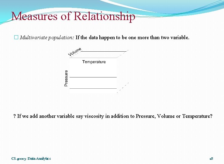
Measures of Relationship � Multivariate population: If the data happen to be one more than two variable. ? If we add another variable say viscosity in addition to Pressure, Volume or Temperature? CS 40003: Data Analytics 18

Measures of Relationship In case of bivariate and multivariate populations, usually, we have to answer two types of questions: Q 1: Does there exist correlation (i. e. , association) between two (or more) variables? If yes, of what degree? Q 2: Is there any cause and effect relationship between the two variables (in case of bivariate population) or one variable in one side and two or more variables on the other side (in case of multivariate population)? If yes, of what degree and in which direction? To find solutions to the above questions, two approaches are known. � Correlation Analysis � Regression Analysis CS 40003: Data Analytics 19

Correlation Analysis CS 40003: Data Analytics 20

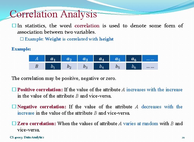
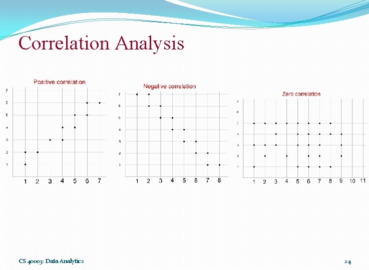
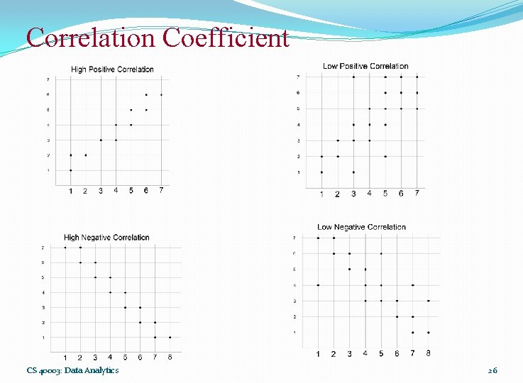
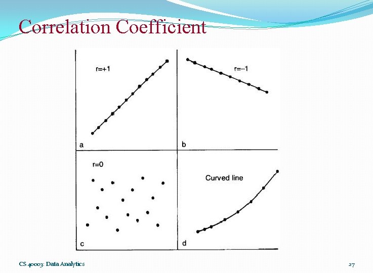
Correlation Analysis � In statistics, the word correlation is used to denote some form of association between two variables. � Example: Weight is correlated with height Example: The correlation may be positive, negative or zero. � Positive correlation: If the value of the attribute A increases with the increase in the value of the attribute B and vice-versa. � Negative correlation: If the value of the attribute A decreases with the increase in the value of the attribute B and vice-versa. � Zero correlation: When the values of attribute A varies at random with B and vice-versa. CS 40003: Data Analytics 21

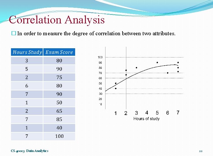
Correlation Analysis � In order to measure the degree of correlation between two attributes. CS 40003: Data Analytics 22

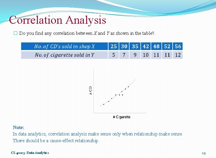
Correlation Analysis � Do you find any correlation between X and Y as shown in the table? . Note: In data analytics, correlation analysis make sense only when relationship make sense. There should be a cause-effect relationship. CS 40003: Data Analytics 23

Correlation Analysis CS 40003: Data Analytics 24

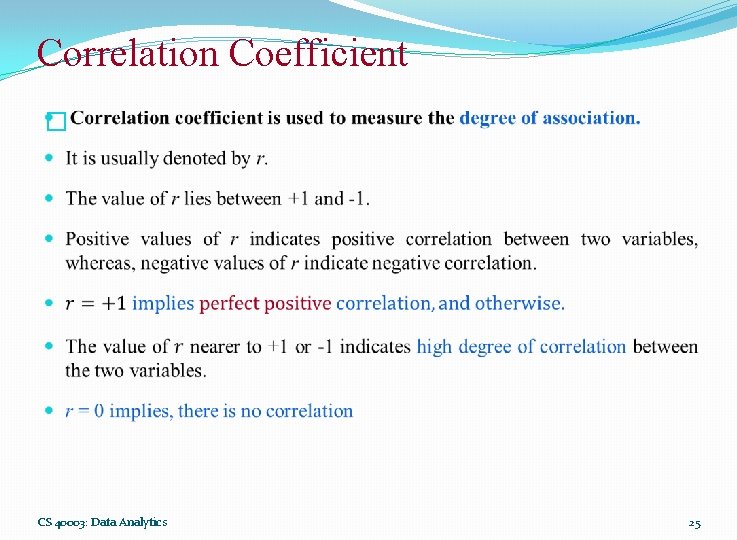
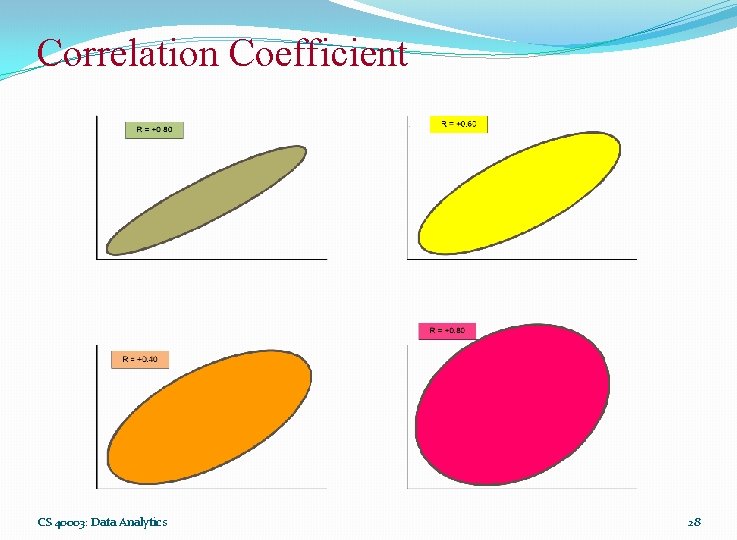
Correlation Coefficient � CS 40003: Data Analytics 25

Correlation Coefficient CS 40003: Data Analytics 26

Correlation Coefficient CS 40003: Data Analytics 27

Correlation Coefficient CS 40003: Data Analytics 28

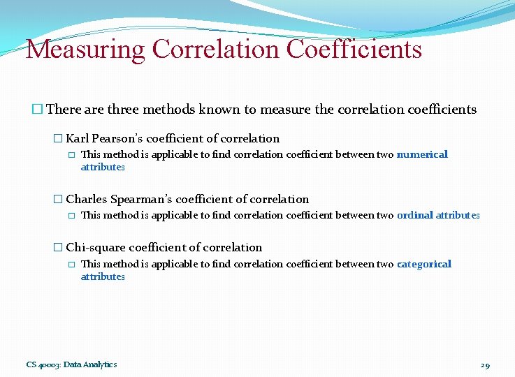
Measuring Correlation Coefficients � There are three methods known to measure the correlation coefficients � Karl Pearson’s coefficient of correlation � This method is applicable to find correlation coefficient between two numerical attributes � Charles Spearman’s coefficient of correlation � This method is applicable to find correlation coefficient between two ordinal attributes � Chi-square coefficient of correlation � This method is applicable to find correlation coefficient between two categorical attributes CS 40003: Data Analytics 29

Pearson’s Correlation Coefficient CS 40003: Data Analytics 30

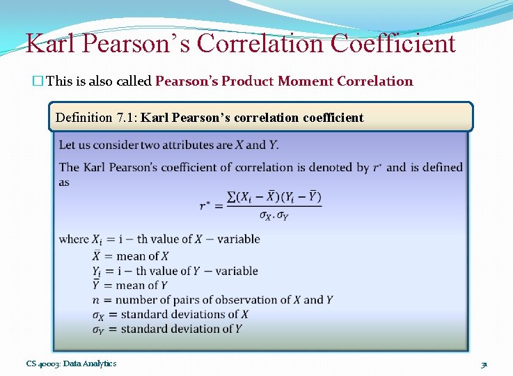
Karl Pearson’s Correlation Coefficient � This is also called Pearson’s Product Moment Correlation Definition 7. 1: Karl Pearson’s correlation coefficient CS 40003: Data Analytics 31

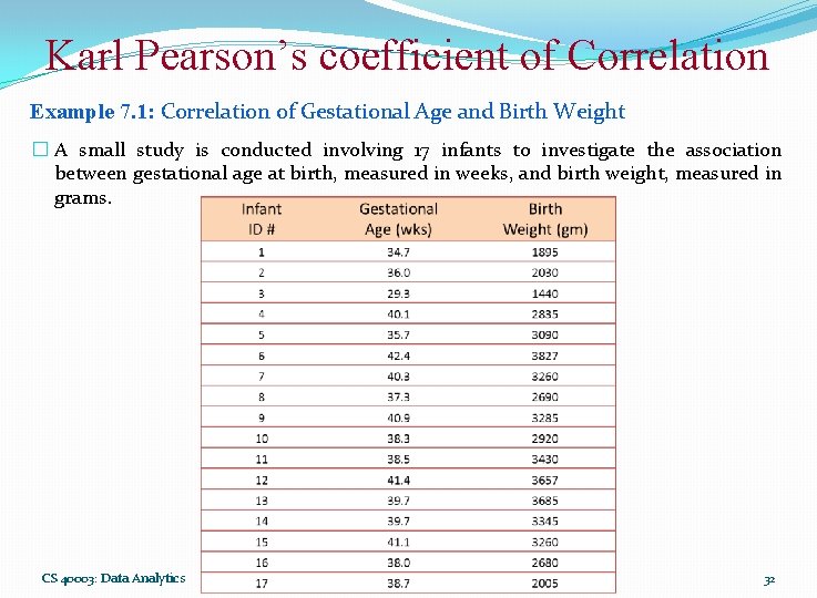
Karl Pearson’s coefficient of Correlation Example 7. 1: Correlation of Gestational Age and Birth Weight � A small study is conducted involving 17 infants to investigate the association between gestational age at birth, measured in weeks, and birth weight, measured in grams. CS 40003: Data Analytics 32

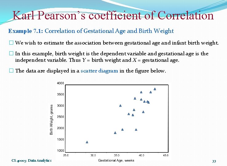
Karl Pearson’s coefficient of Correlation Example 7. 1: Correlation of Gestational Age and Birth Weight � We wish to estimate the association between gestational age and infant birth weight. � In this example, birth weight is the dependent variable and gestational age is the independent variable. Thus Y = birth weight and X = gestational age. � The data are displayed in a scatter diagram in the figure below. CS 40003: Data Analytics 33

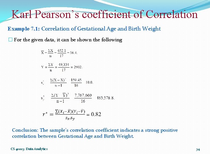
Karl Pearson’s coefficient of Correlation Example 7. 1: Correlation of Gestational Age and Birth Weight � For the given data, it can be shown the following Conclusion: The sample’s correlation coefficient indicates a strong positive correlation between Gestational Age and Birth Weight. CS 40003: Data Analytics 34

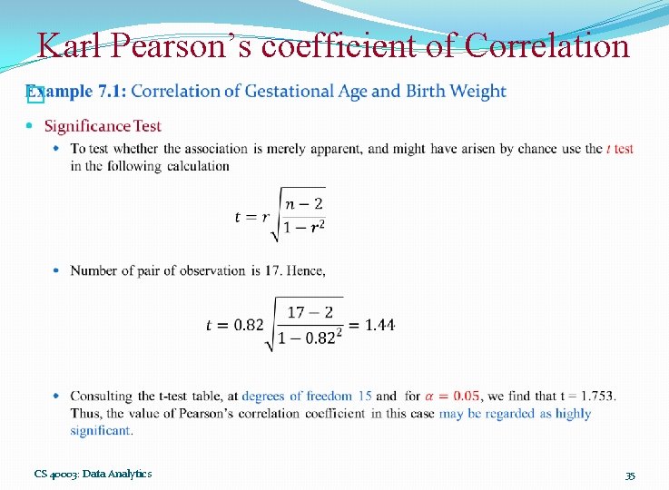
Karl Pearson’s coefficient of Correlation � CS 40003: Data Analytics 35

Rank Correlation Coefficient CS 40003: Data Analytics 36

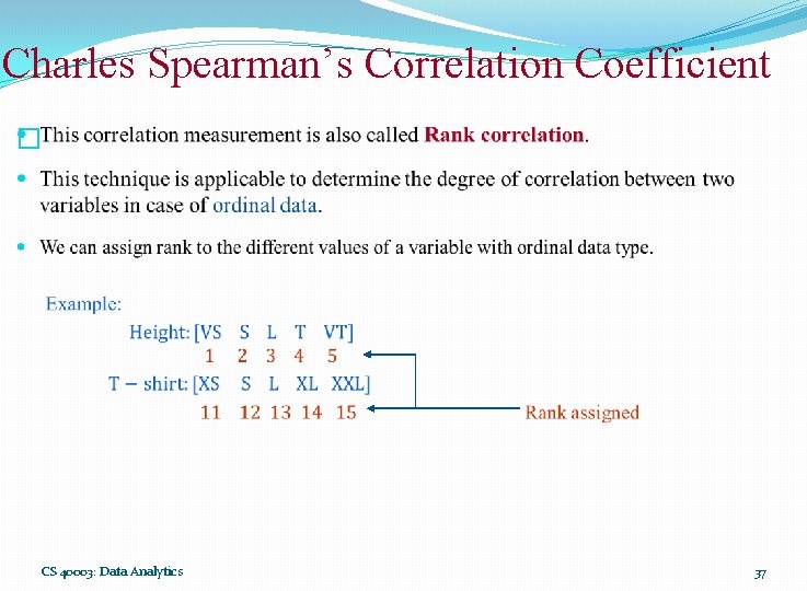
Charles Spearman’s Correlation Coefficient � CS 40003: Data Analytics 37

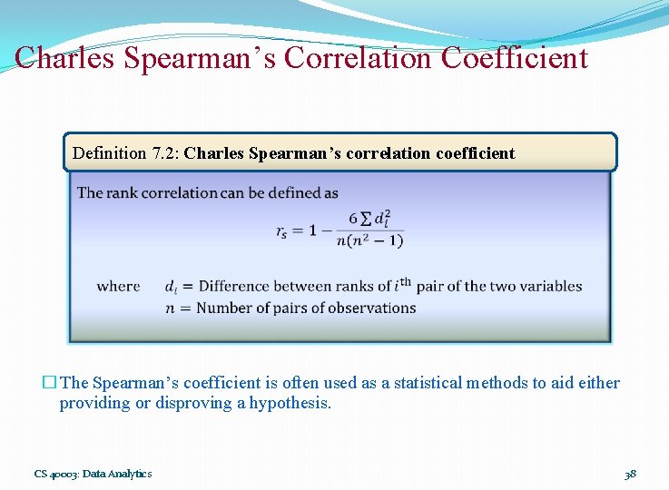
Charles Spearman’s Correlation Coefficient Definition 7. 2: Charles Spearman’s correlation coefficient � The Spearman’s coefficient is often used as a statistical methods to aid either providing or disproving a hypothesis. CS 40003: Data Analytics 38

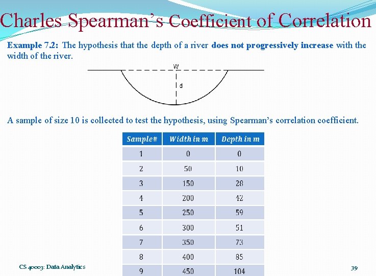
Charles Spearman’s Coefficient of Correlation Example 7. 2: The hypothesis that the depth of a river does not progressively increase with the width of the river. A sample of size 10 is collected to test the hypothesis, using Spearman’s correlation coefficient. CS 40003: Data Analytics 39

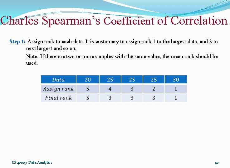
Charles Spearman’s Coefficient of Correlation Step 1: Assign rank to each data. It is customary to assign rank 1 to the largest data, and 2 to next largest and so on. Note: If there are two or more samples with the same value, the mean rank should be used. CS 40003: Data Analytics 40

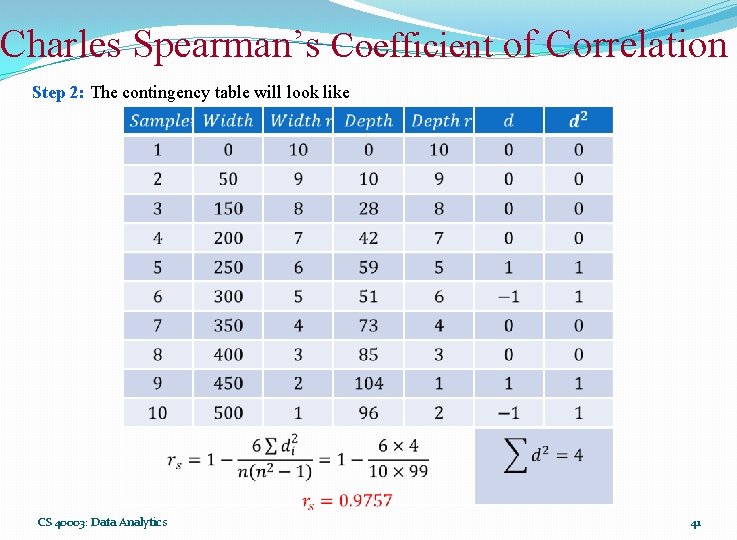
Charles Spearman’s Coefficient of Correlation Step 2: The contingency table will look like CS 40003: Data Analytics 41

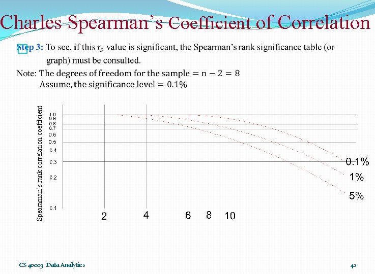
Charles Spearman’s Coefficient of Correlation Spearaman’s rank correlation coefficient � CS 40003: Data Analytics 42

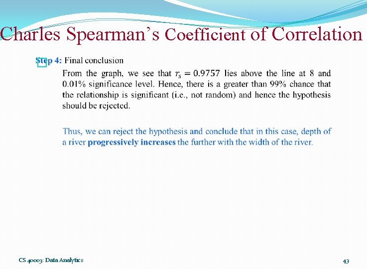
Charles Spearman’s Coefficient of Correlation � CS 40003: Data Analytics 43

χ2 -Correlation Analysis CS 40003: Data Analytics 44

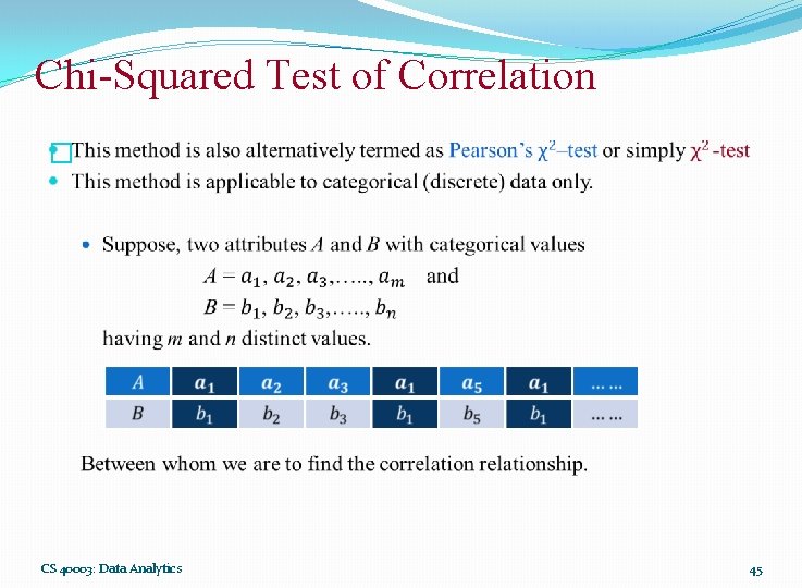
Chi-Squared Test of Correlation � CS 40003: Data Analytics 45

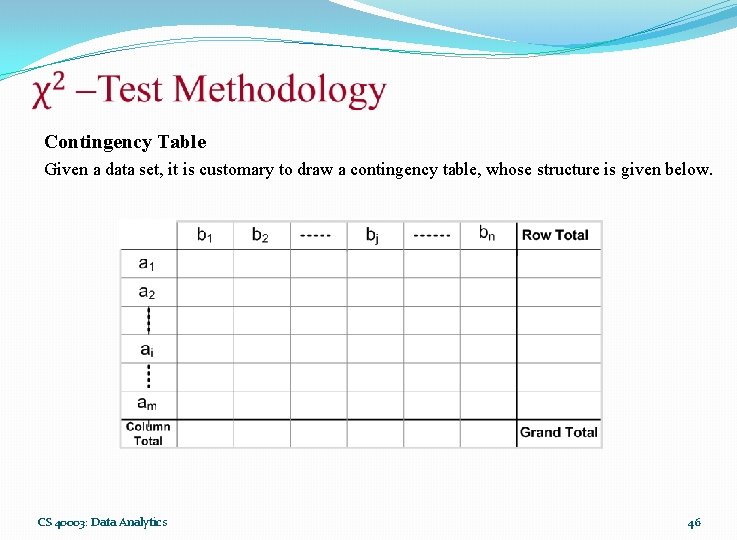
Contingency Table Given a data set, it is customary to draw a contingency table, whose structure is given below. CS 40003: Data Analytics 46

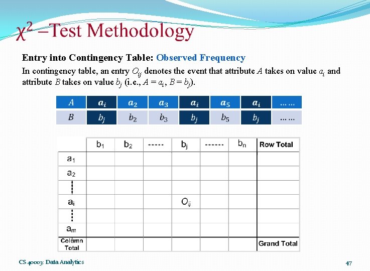
Entry into Contingency Table: Observed Frequency In contingency table, an entry Oij denotes the event that attribute A takes on value ai and attribute B takes on value bj (i. e. , A = ai, B = bj). CS 40003: Data Analytics 47

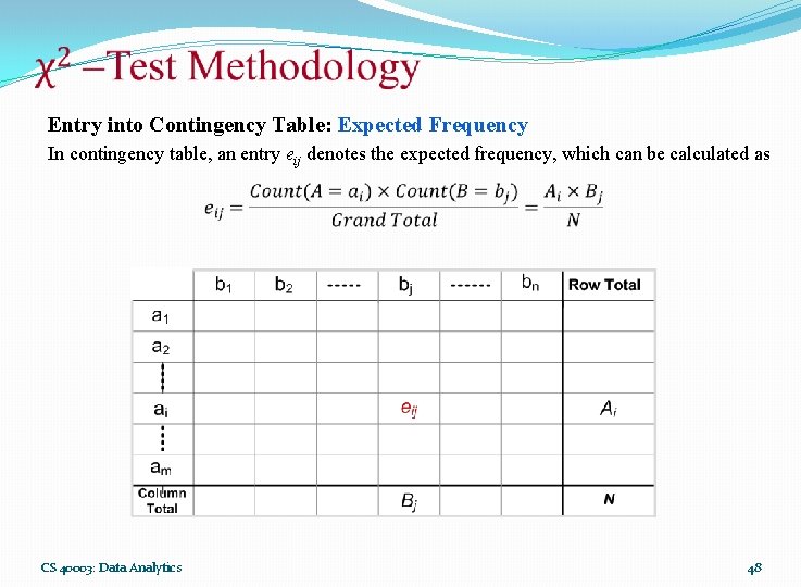
Entry into Contingency Table: Expected Frequency In contingency table, an entry eij denotes the expected frequency, which can be calculated as CS 40003: Data Analytics 48

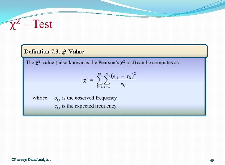
Definition 7. 3: χ2 -Value CS 40003: Data Analytics 49

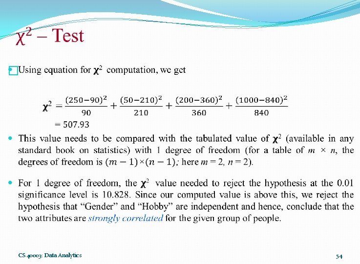
2 value are those whose � The cell that contribute the most to the �� actual count is very different from the expected. 2 statistics tests the hypothesis that A and B are independent. � The �� The test is based on a significance level, with (n-1) ×(m-1) degrees of freedom. , with a contingency table of size n×m � If the hypothesis can be rejected, then we say that A and B are statistically related or associated. CS 40003: Data Analytics 50

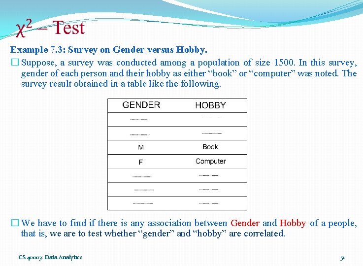
Example 7. 3: Survey on Gender versus Hobby. � Suppose, a survey was conducted among a population of size 1500. In this survey, gender of each person and their hobby as either “book” or “computer” was noted. The survey result obtained in a table like the following. � We have to find if there is any association between Gender and Hobby of a people, that is, we are to test whether “gender” and “hobby” are correlated. CS 40003: Data Analytics 51

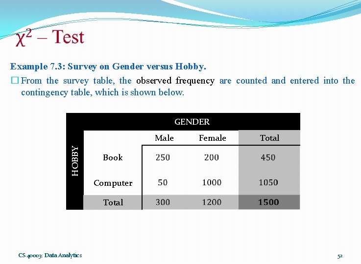
Example 7. 3: Survey on Gender versus Hobby. � From the survey table, the observed frequency are counted and entered into the contingency table, which is shown below. GENDER HOBBY Male Female Total Book Computer Total CS 40003: Data Analytics 52

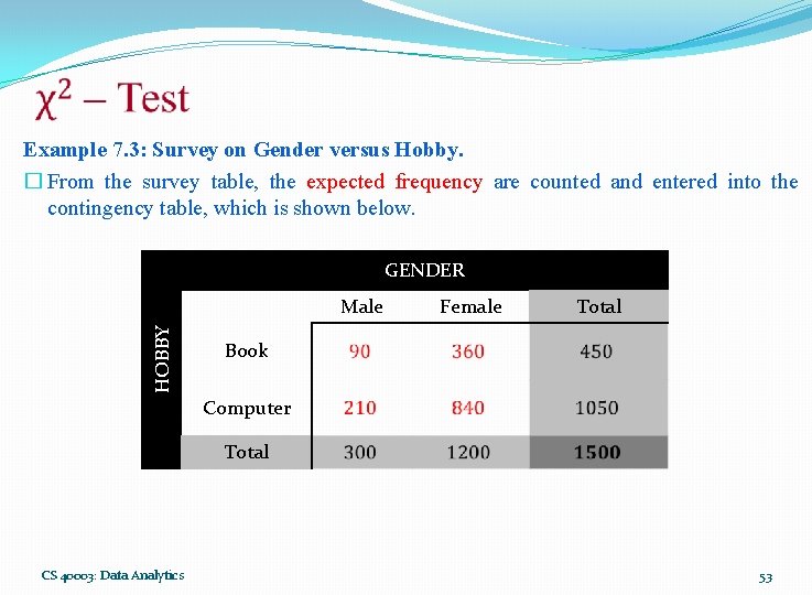
Example 7. 3: Survey on Gender versus Hobby. � From the survey table, the expected frequency are counted and entered into the contingency table, which is shown below. GENDER HOBBY Male Female Total Book Computer Total CS 40003: Data Analytics 53

� CS 40003: Data Analytics 54

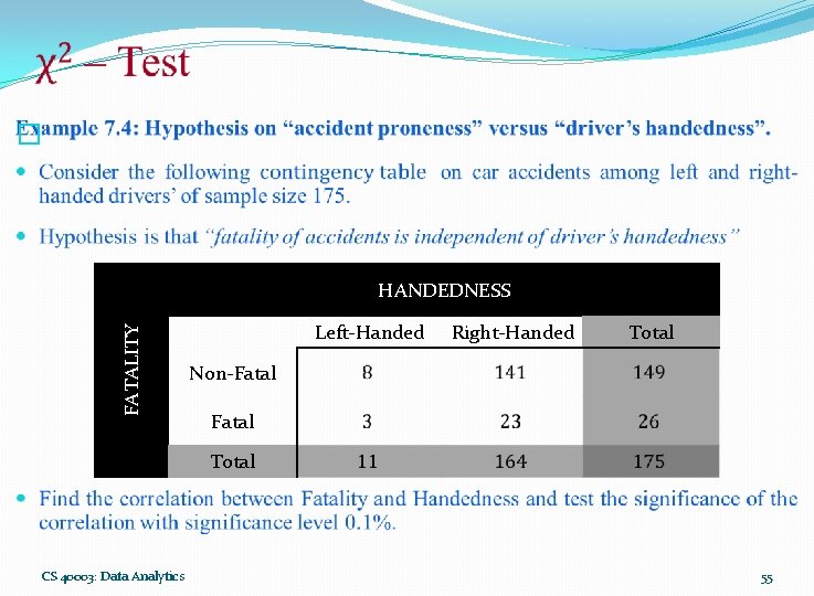
� FATALITY HANDEDNESS Left-Handed Right-Handed Total Non-Fatal Total CS 40003: Data Analytics 55

Regression Analysis CS 40003: Data Analytics 56

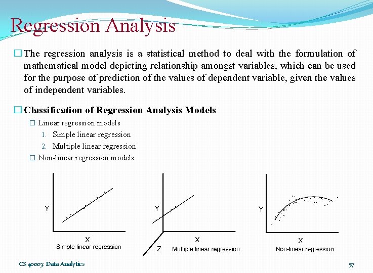
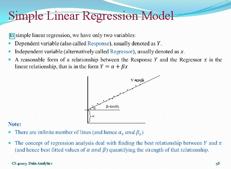
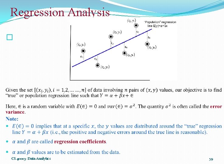
Regression Analysis � The regression analysis is a statistical method to deal with the formulation of mathematical model depicting relationship amongst variables, which can be used for the purpose of prediction of the values of dependent variable, given the values of independent variables. � Classification of Regression Analysis Models � Linear regression models 1. Simple linear regression 2. Multiple linear regression � Non-linear regression models CS 40003: Data Analytics 57

Simple Linear Regression Model � CS 40003: Data Analytics 58

Regression Analysis � CS 40003: Data Analytics 59

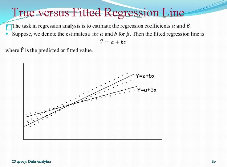
True versus Fitted Regression Line � CS 40003: Data Analytics 60

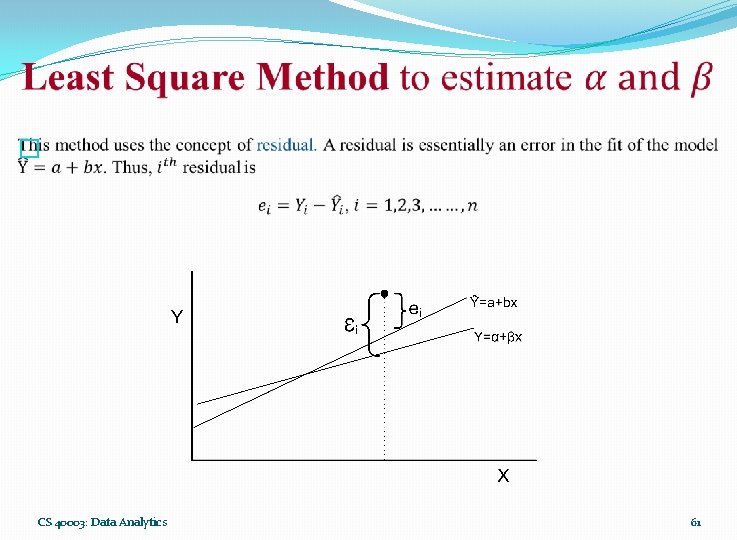
� CS 40003: Data Analytics 61

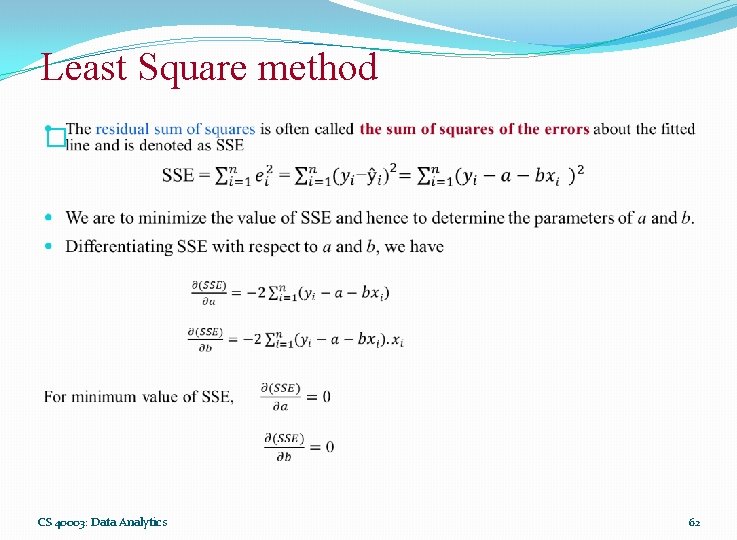
Least Square method � CS 40003: Data Analytics 62

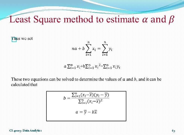
� CS 40003: Data Analytics 63

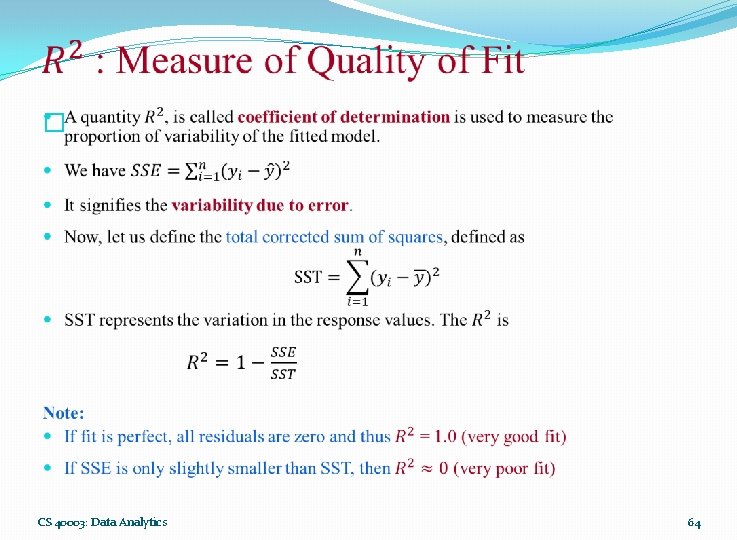
� CS 40003: Data Analytics 64

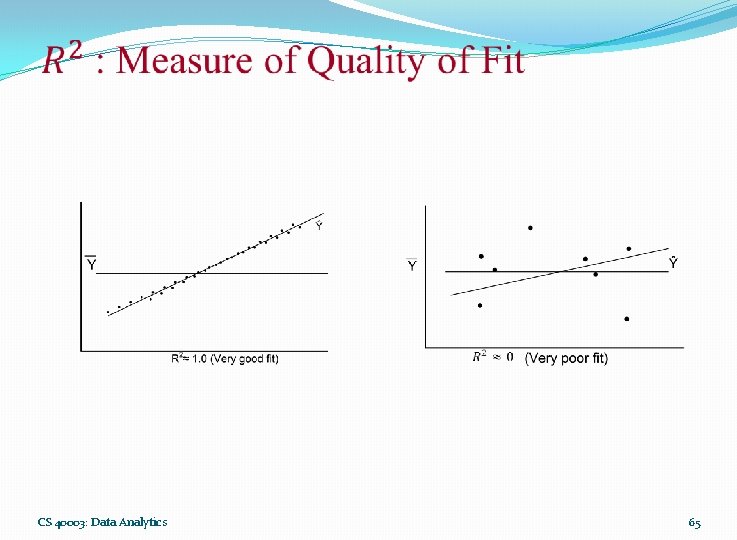
CS 40003: Data Analytics 65

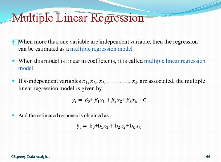
Multiple Linear Regression � CS 40003: Data Analytics 66

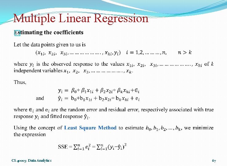
Multiple Linear Regression � CS 40003: Data Analytics 67

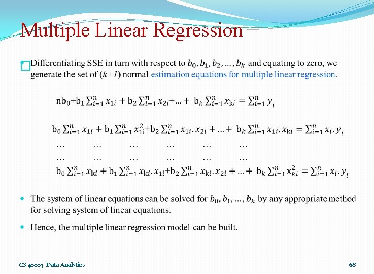
Multiple Linear Regression � CS 40003: Data Analytics 68

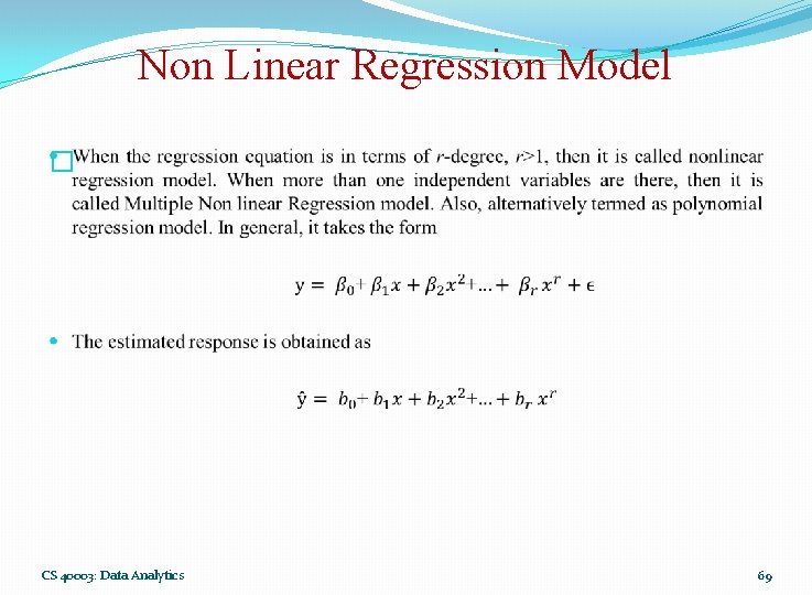
Non Linear Regression Model � CS 40003: Data Analytics 69

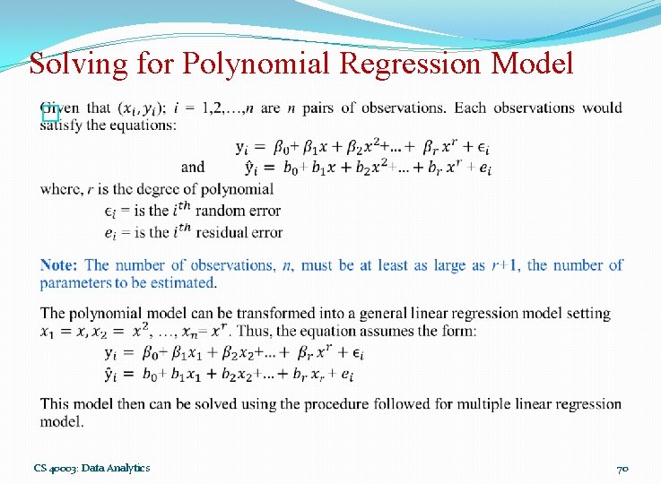
Solving for Polynomial Regression Model � CS 40003: Data Analytics 70

Auto-Regression Analysis CS 40003: Data Analytics 71

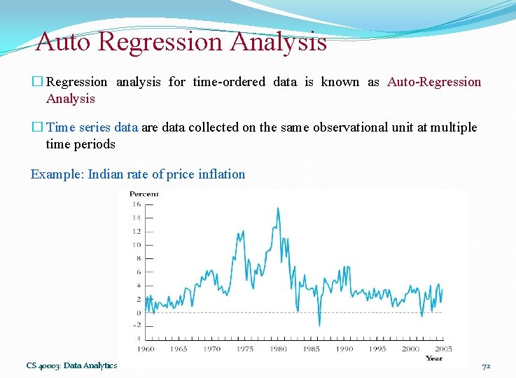
Auto Regression Analysis � Regression analysis for time-ordered data is known as Auto-Regression Analysis � Time series data are data collected on the same observational unit at multiple time periods Example: Indian rate of price inflation CS 40003: Data Analytics 72

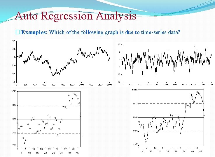
Auto Regression Analysis � Examples: Which of the following is a time-series data? � Aggregate consumption and GDP for a country (for example, 20 years of quarterly observations = 80 observations) � Yen/$, pound/$ and Euro/$ exchange rates (daily data for 1 year = 365 observations) � Cigarette consumption per capita in a state, by years � Rainfall data over a year � Sales of tea from a tea shop in a season CS 40003: Data Analytics 73

Auto Regression Analysis � Examples: Which of the following graph is due to time-series data? CS 40003: Data Analytics 74

Use of Time Series Data � To develop forecast model � What will the rate of inflation be next year? � To estimate dynamic causal effects � If the rate of interest increases the interest rate now, what will be the effect on the rates of inflation and unemployment in 3 months? in 12 months? � What is the effect over time on electronics good consumption of a hike in the excise duty? � Time dependent analysis � Rates of inflation and unemployment in the country can be observed only over time! CS 40003: Data Analytics 75

Modeling with Time Series Data � Correlation over time � Serial correlation, also called autocorrelation � Calculating standard error � To estimate dynamic causal effects � Under which dynamic effects can be estimated? � How to estimate? � Forecasting model build on regression model CS 40003: Data Analytics 76

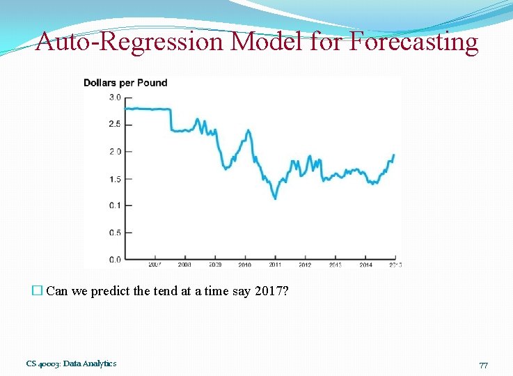
Auto-Regression Model for Forecasting � Can we predict the tend at a time say 2017? CS 40003: Data Analytics 77

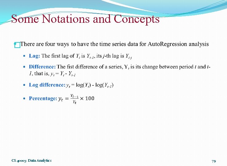
Some Notations and Concepts � Yt = Value of Y in a period t � Data set [Y 1, Y 2, … YT-1, YT]: T observations on the time series random variable Y � Assumptions � We consider only consecutive, evenly spaced observations � For example, monthly, 2000 -2015, no missing months � A time series Yt is stationary if its probability distribution does not change over time, that is, if the joint distribution of (Yi+1, Yi+2, …, Yi+T) does not depend on i. � Stationary property implies that history is relevant. In other words, Stationary requires the future to be like the past (in a probabilistic sense). � Auto Regression analysis assumes that Yt is stationary. CS 40003: Data Analytics 78

Some Notations and Concepts � CS 40003: Data Analytics 79

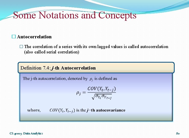
Some Notations and Concepts � Autocorrelation � The correlation of a series with its own lagged values is called autocorrelation (also called serial correlation) Definition 7. 4: j-th Autocorrelation CS 40003: Data Analytics 80

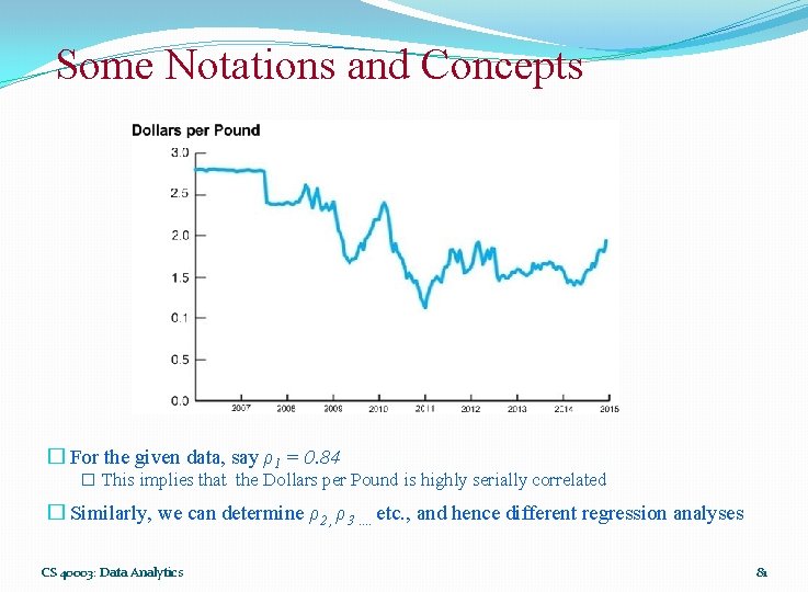
Some Notations and Concepts � For the given data, say ρ1 = 0. 84 � This implies that the Dollars per Pound is highly serially correlated � Similarly, we can determine ρ2 , ρ3 …. etc. , and hence different regression analyses CS 40003: Data Analytics 81

Auto-Regression Model for Forecatsing � A natural starting point forecasting model is to use past values of Y, that is, Yt-1, Yt-2, … to predict Yt � An autoregression is a regression model in which Yt is regressed against its own lagged values. � The number of lags used as regressors is called the order of autoregression � In first order autoregression (denoted as AR(1)), Yt is regressed against Yt-1 � In p-th order autoregression (denoted as AR(p)), Yt is regressed against, Yt-1, Yt-2, …, Yt-p CS 40003: Data Analytics 82

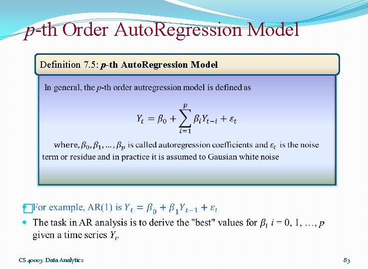
p-th Order Auto. Regression Model Definition 7. 5: p-th Auto. Regression Model � CS 40003: Data Analytics 83

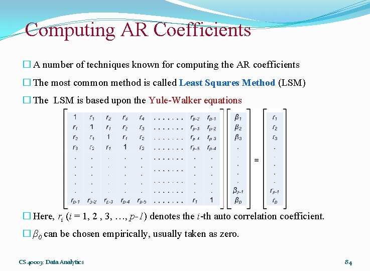
Computing AR Coefficients � A number of techniques known for computing the AR coefficients � The most common method is called Least Squares Method (LSM) � The LSM is based upon the Yule-Walker equations � Here, ri (i = 1, 2 , 3, …, p-1) denotes the i-th auto correlation coefficient. � β 0 can be chosen empirically, usually taken as zero. CS 40003: Data Analytics 84

Reference �The detail material related to this lecture can be found in The Elements of Statistical Learning, Data Mining, Inference, and Prediction (2 nd Edn. ), Trevor Hastie, Robert Tibshirani, Jerome Friedman, Springer, 2014. CS 40003: Data Analytics 85

Any question? You may post your question(s) at the “Discussion Forum” maintained in the course Web page! CS 40003: Data Analytics 86

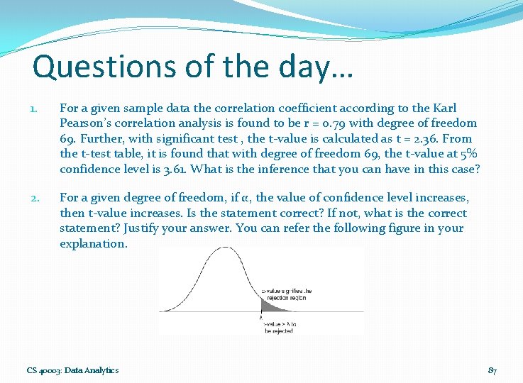
Questions of the day… 1. For a given sample data the correlation coefficient according to the Karl Pearson’s correlation analysis is found to be r = 0. 79 with degree of freedom 69. Further, with significant test , the t-value is calculated as t = 2. 36. From the t-test table, it is found that with degree of freedom 69, the t-value at 5% confidence level is 3. 61. What is the inference that you can have in this case? 2. For a given degree of freedom, if α, the value of confidence level increases, then t-value increases. Is the statement correct? If not, what is the correct statement? Justify your answer. You can refer the following figure in your explanation. CS 40003: Data Analytics 87

Questions of the day… � CS 40003: Data Analytics 88