Data Analytics CS 40003 Lecture 12 Clustering Techniques
 Lecture #12 Clustering Techniques: Similarity Measures Dr. Debasis Samanta Associate")


 is an important")


 at the “Discussion Forum” maintained in the")
- Slides: 48
Data Analytics (CS 40003) Lecture #12 Clustering Techniques: Similarity Measures Dr. Debasis Samanta Associate Professor Department of Computer Science & Engineering
Topics to be covered… � Introduction to clustering � Similarity and dissimilarity measures � Clustering techniques � Partitioning algorithms � Hierarchical algorithms � Density-based algorithm CS 40003: Data Analytics 2
Introduction to Clustering � Classification consists of assigning a class label to a set of unclassified cases. � Supervised Classification � The set of possible classes is known in advance. � Unsupervised Classification � Set of possible classes is not known. After classification we can try to assign a name to that class. � Unsupervised classification is called clustering. CS 40003: Data Analytics 3
Supervised Technique CS 40003: Data Analytics 4
Unsupervised Technique CS 40003: Data Analytics 5
Introduction to Clustering � Clustering is somewhat related to classification in the sense that in both cases data are grouped. • � However, there is a major difference between these two techniques. � In order to understand the difference between the two, consider a sample dataset containing marks obtained by a set of students and corresponding grades as shown in Table 15. 1. CS 40003: Data Analytics 6
Introduction to Clustering Table 12. 1: Tabulation of Marks Roll No Mark Grade 1 80 A 2 70 A 3 55 C 4 91 EX 5 65 B 6 35 D 7 76 A 8 40 D 9 50 C 10 85 EX 11 25 F 12 60 B 13 45 D 14 95 EX 15 63 B 16 88 A CS 40003: Data Analytics Figure 12. 1: Group representation of dataset in Table 15. 1 F B EX 11 5 4 12 15 C 3 D 8 6 10 14 9 13 1 16 2 A 7 7
Introduction to Clustering � It is evident that there is a simple mapping between Table 12. 1 and Fig 12. 1. � The fact is that groups in Fig 12. 1 are already predefined in Table 12. 1. This is similar to classification, where we have given a dataset where groups of data are predefined. � Consider another situation, where ‘Grade’ is not known, but we have to make a grouping. � Put all the marks into a group if any other mark in that group does not exceed by 5 or more. � This is similar to “Relative grading” concept and grade may range from A to Z. CS 40003: Data Analytics 8
Introduction to Clustering � Figure 12. 2 shows another grouping by means of another simple mapping, but the difference is this mapping does not based on predefined classes. � In other words, this grouping is accomplished by finding similarities between data according to characteristics found in the actual data. � Such a group making is called clustering.
Introduction to Clustering Example 12. 1 : The task of clustering In order to elaborate the clustering task, consider the following dataset. Table 12. 2: Life Insurance database Martial Status Single Age Income Education 35 25000 Under Graduate Number of children 3 Married 25 15000 Graduate 1 Single 40 20000 Under Graduate 0 Divorced 20 30000 Post-Graduate 0 Divorced 25 20000 Under Graduate 3 Married 60 70000 Graduate 0 Married 30 90000 Post-Graduate 0 Married 45 60000 Graduate 5 Divorced 50 80000 Under Graduate 2 With certain similarity or likeliness defined, we can classify the records to one or group of more attributes (and thus mapping being non-trivial). CS 40003: Data Analytics 10
Introduction to Clustering � Clustering has been used in many application domains: � Image analysis � Document retrieval � Machine learning, etc. � When clustering is applied to real-world database, many problems may arise. 1. The (best) number of cluster is not known. � There is not correct answer to a clustering problem. � In fact, many answers may be found. � The exact number of cluster required is not easy to determine. CS 40003: Data Analytics 11
Introduction to Clustering 2. There may not be any a priori knowledge concerning the clusters. • This is an issue that what data should be used for clustering. • Unlike classification, in clustering, we have not supervisory learning to aid the process. • Clustering can be viewed as similar to unsupervised learning. 3. Interpreting the semantic meaning of each cluster may be difficult. • With classification, the labeling of classes is known ahead of time. In contrast, with clustering, this may not be the case. • Thus, when the clustering process is finished yielding a set of clusters, the exact meaning of each cluster may not be obvious. CS 40003: Data Analytics 12
Definition of Clustering Problem Definition 12. 1: Clustering • Solution to a clustering problem is devising a mapping formulation. • The formulation behind such a mapping is to establish that a tuple within one cluster is more like tuples within that cluster and not similar to tuples outside it. CS 40003: Data Analytics 13
Definition of Clustering Problem CS 40003: Data Analytics 14
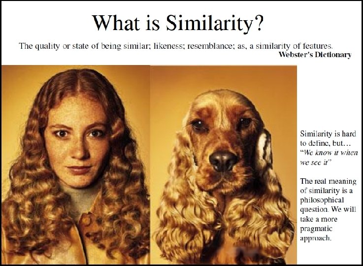
Similarity and Dissimilarity Measures • In clustering techniques, similarity (or dissimilarity) is an important measurement. • Informally, similarity between two objects (e. g. , two images, two documents, two records, etc. ) is a numerical measure of the degree to which two objects are alike. • The dissimilarity on the other hand, is another alternative (or opposite) measure of the degree to which two objects are different. • Both similarity and dissimilarity also termed as proximity. • Usually, similarity and dissimilarity are non-negative numbers and may range from zero (highly dissimilar (no similar)) to some finite/infinite value (highly similar (no dissimilar)). Note: • Frequently, the term distance is used as a synonym for dissimilarity • In fact, it is used to refer as a special case of dissimilarity. CS 40003: Data Analytics 16
Proximity Measures: Single-Attribute CS 40003: Data Analytics 17
Proximity Calculation � Object Gender Ram Male Sita Female Laxman Male CS 40003: Data Analytics 18
Proximity Calculation Table 12. 3: Contingency table with binary attributes Object �� 1 0 CS 40003: Data Analytics 19
Similarity Measure with Symmetric Binary CS 40003: Data Analytics 20
Similarity Measure with Symmetric Binary Example 12. 2: Proximity measures with symmetric binary attributes Consider the following two dataset, where objects are defined with symmetric binary attributes. Gender = {M, F}, Food = {V, N}, Hobby = {T, C}, Job = {Y, N} Caste = {H, M}, Education = {L, I}, Object Gender Food Caste Education Hobby Job Hari M V M L C N Ram M N M I T N Tomi F N H L C Y CS 40003: Data Analytics 21
Proximity Measure with Asymmetric Binary CS 40003: Data Analytics 22
Proximity Measure with Asymmetric Binary Example 12. 3: Jaccard Coefficient Consider the following two dataset. Gender = {M, F}, Food = {V, N}, Caste = {H, M}, Hobby = {T, C}, Job = {Y, N} Education = {L, I}, Calculate the Jaccard coefficient between Ram and Hari assuming that all binary attributes are asymmetric and for each pair values for an attribute, first one is more frequent than the second. Object Gender Food Caste Education Hobby Job Hari M V M L C N Ram M N M I T N Tomi F N H L C Y CS 40003: Data Analytics 23
Example 12. 4: Consider the following two dataset. Gender = {M, F}, Food = {V, N}, Caste = {H, M}, Hobby = {T, C}, Job = {Y, N} ? Education = {L, I}, Object Gender Food Caste Education Hobby Job Hari M V M L C N Ram M N M I T N Tomi F N H L C Y How you can calculate similarity if Gender, Hobby and Job are symmetric binary attributes and Food, Caste, Education are asymmetric binary attributes? Obtain the similarity matrix with Jaccard coefficient of objects for the above, e. g. CS 40003: Data Analytics 24
Proximity Measure with Categorical Attribute CS 40003: Data Analytics 25
Proximity Measure with Categorical Attribute Example 12. 4: Object Color Position Distance 1 R L L 2 B C M 3 G R M 4 R L H The similarity matrix considering only color attribute is shown below Obtain the dissimilarity matrix considering both the categorical attributes (i. e. color and position). CS 40003: Data Analytics 26
Proximity Measure with Ordinal Attribute CS 40003: Data Analytics 27
Proximity Measure with Ordinal Attribute Example 12. 5: Consider the following set of records, where each record is defined by two ordinal attributes size={S, M, L} and Quality = {Ex, A, B, C} such that S<M<L and Ex>A>B>C. Object Size Quality A S (0. 0) A (0. 66) B L (1. 0) Ex (1. 0) C L (1. 0) C (0. 0) D M (0. 5) B (0. 33) • Normalized values are shown in brackets. • Their similarity measures are shown in the similarity matrix below. ? Find the dissimilarity matrix, when each object is defined by only one ordinal attribute say size (or quality). CS 40003: Data Analytics 28
Proximity Measure with Interval Scale CS 40003: Data Analytics 29
Proximity Measure with Interval Scale CS 40003: Data Analytics 30
Proximity Measure with Interval Scale CS 40003: Data Analytics 31
Proximity Measure with Interval Scale CS 40003: Data Analytics 32
Proximity Measure with Interval Scale CS 40003: Data Analytics 33
Proximity Measure with Interval Scale CS 40003: Data Analytics 34
Proximity Measure for Ratio-Scale CS 40003: Data Analytics 35
Proximity Measure for Ratio-Scale CS 40003: Data Analytics 36
Proximity Measure for Ratio-Scale CS 40003: Data Analytics 37
Proximity Measure with Mixed Attributes • The previous metrics on similarity measures assume that all the attributes were of the same type. Thus, a general approach is needed when the attributes are of different types. • One straightforward approach is to compute the similarity between each attribute separately and then combine these attribute using a method that results in a similarity between 0 and 1. • Typically, the overall similarity is defined as the average of all the individual attribute similarities. • See the algorithm in the next slide for doing this. CS 40003: Data Analytics 38
Similarity Measure with Vector Objects CS 40003: Data Analytics 39
Similarity Measure with Mixed Attributes Example 12. 6: Consider the following set of objects. Obtain the similarity matrix. Object A (Binary) B (Categorical) C (Ordinal) D (Numeric) E (Numeric) 1 Y R X 475 108 2 N R A 10 10 -2 3 N B C 1000 105 4 Y G B 500 103 5 Y B A 80 1 [For C: X>A>B>C] How cosine similarity can be applied to this? CS 40003: Data Analytics 40
Non-Metric similarity CS 40003: Data Analytics 41
Cosine Similarity CS 40003: Data Analytics 42
Non-Metric Similarity CS 40003: Data Analytics 43
Pearson’s Correlation CS 40003: Data Analytics 44
CS 40003: Data Analytics 45
Mahalanobis Distance CS 40003: Data Analytics 46
Set Difference and Time Difference CS 40003: Data Analytics 47
Any question? You may post your question(s) at the “Discussion Forum” maintained in the course Web page! CS 40003: Data Analytics 48