Data Analytics CS 40003 Lecture 4 Programming with

Data Analytics (CS 40003) Lecture #4 Programming with R Dr. Debasis Samanta Associate Professor Department of Computer Science & Engineering

Quote of the day. . �What we think, we become. � GAUTAMA CS 40003: Data Analytics BUDDHA, Sege 2

Today’s discussion… � R is an open source programming language and software environment for statistical computing and graphics. � The R language is widely used among statisticians and data miners for developing statistical software and data analytics tools CS 40003: Data Analytics 3

History of R �Modelled after S & S-plus, developed at AT&T labs in late 1980 s. �R project was started by Robert Gentleman and Ross Ihaka Department of Statistics, University of Auckland (1995). �Currently maintained by R core development team – an international team of volunteer developers (since 1997).

R resources �http: //www. r-project. org/ �http: //cran. r-project. org/doc/contrib/Verzani-Simple. R. pdf

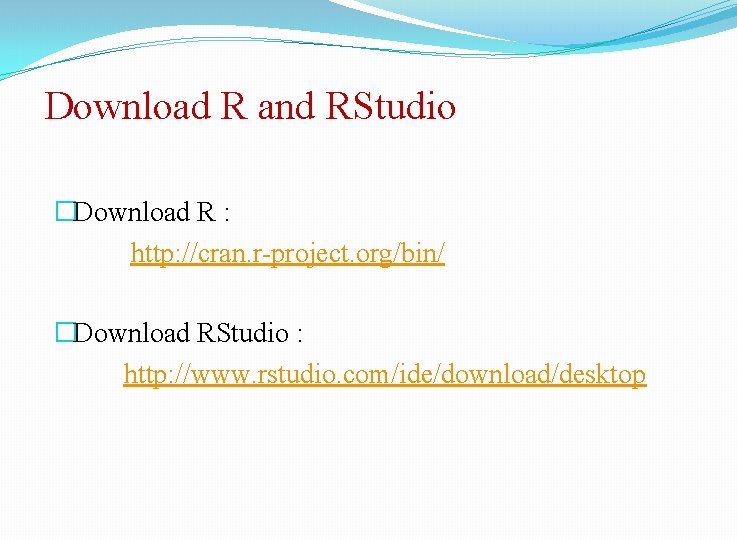
Download R and RStudio �Download R : http: //cran. r-project. org/bin/ �Download RStudio : http: //www. rstudio. com/ide/download/desktop

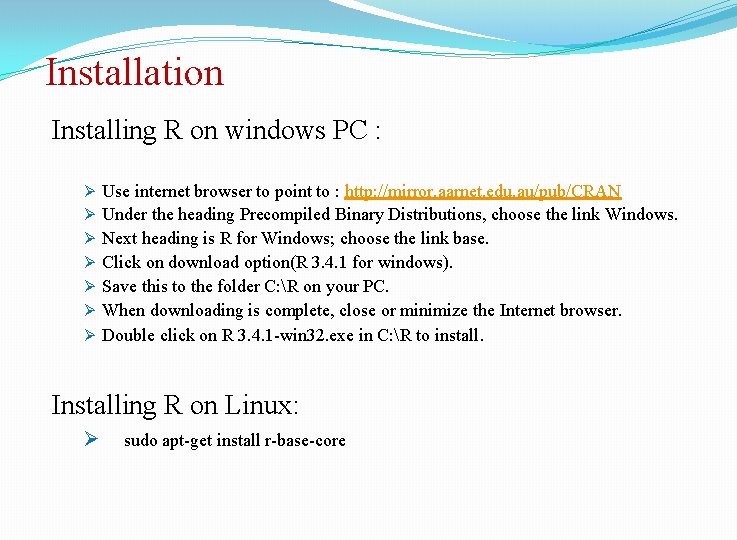
Installation Installing R on windows PC : Ø Use internet browser to point to : http: //mirror. aarnet. edu. au/pub/CRAN Ø Under the heading Precompiled Binary Distributions, choose the link Windows. Ø Next heading is R for Windows; choose the link base. Ø Click on download option(R 3. 4. 1 for windows). Ø Save this to the folder C: R on your PC. Ø When downloading is complete, close or minimize the Internet browser. Ø Double click on R 3. 4. 1 -win 32. exe in C: R to install. Installing R on Linux: Ø sudo apt-get install r-base-core

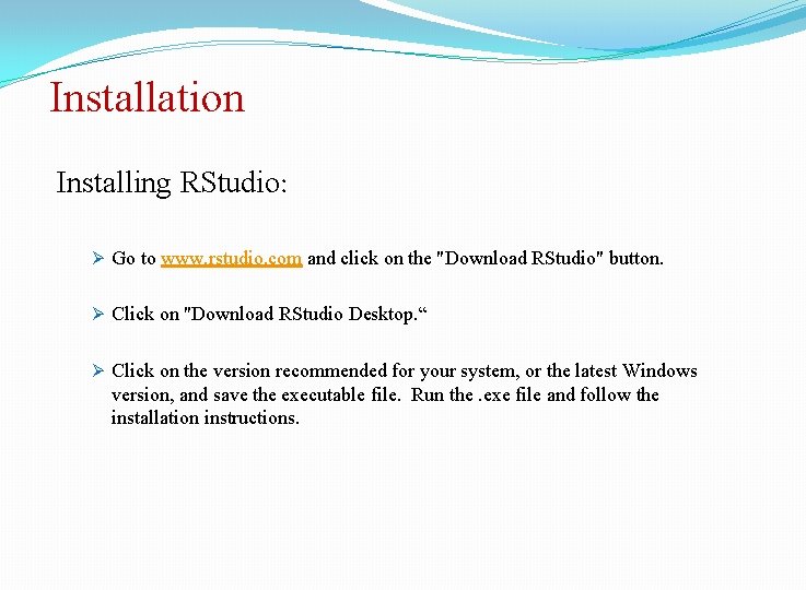
Installation Installing RStudio: Ø Go to www. rstudio. com and click on the "Download RStudio" button. Ø Click on "Download RStudio Desktop. “ Ø Click on the version recommended for your system, or the latest Windows version, and save the executable file. Run the. exe file and follow the installation instructions.

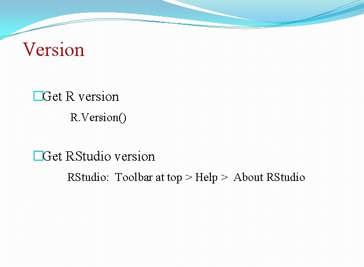
Version �Get R version R. Version() �Get RStudio version RStudio: Toolbar at top > Help > About RStudio

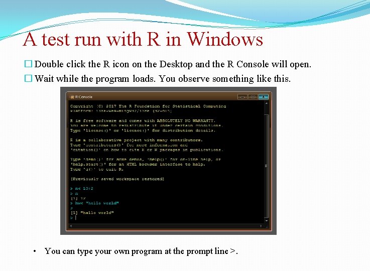
A test run with R in Windows � Double click the R icon on the Desktop and the R Console will open. � Wait while the program loads. You observe something like this. • You can type your own program at the prompt line >.

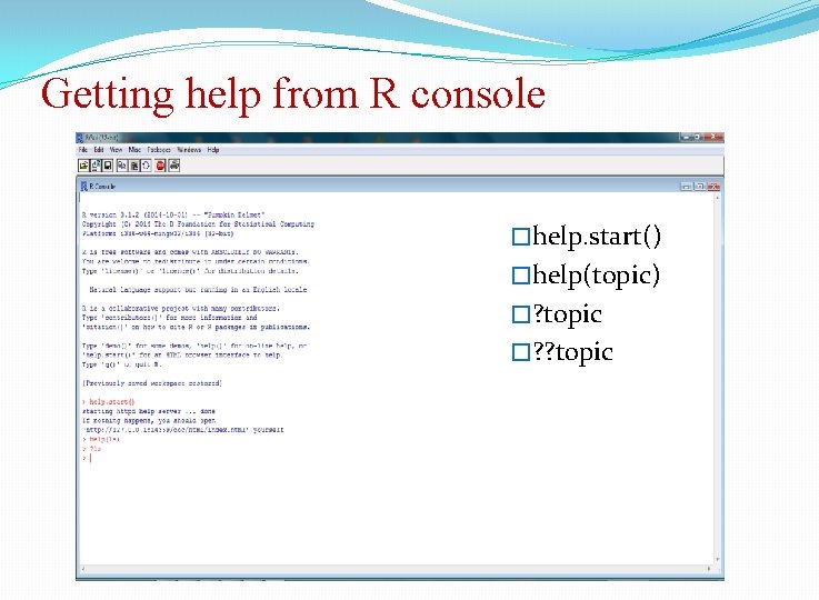
Getting help from R console �help. start() �help(topic) �? topic �? ? topic

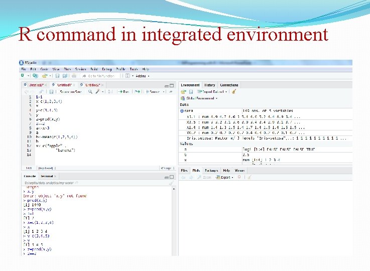
R command in integrated environment

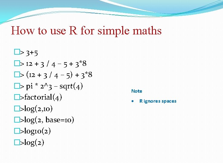
How to use R for simple maths �> 3+5 �> 12 + 3 / 4 – 5 + 3*8 �> (12 + 3 / 4 – 5) + 3*8 �> pi * 2^3 – sqrt(4) �>factorial(4) �>log(2, 10) �>log(2, base=10) �>log 10(2) �>log(2) Note R ignores spaces

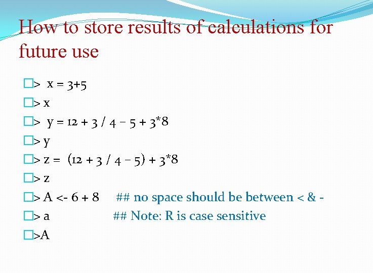
How to store results of calculations for future use �> x = 3+5 �> x �> y = 12 + 3 / 4 – 5 + 3*8 �> y �> z = (12 + 3 / 4 – 5) + 3*8 �> z �> A <- 6 + 8 ## no space should be between < & �> a ## Note: R is case sensitive �>A

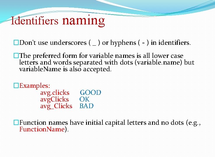
Identifiers naming �Don't use underscores ( _ ) or hyphens ( - ) in identifiers. �The preferred form for variable names is all lower case letters and words separated with dots (variable. name) but variable. Name is also accepted. �Examples: avg. clicks avg. Clicks avg_Clicks GOOD OK BAD �Function names have initial capital letters and no dots (e. g. , Function. Name).

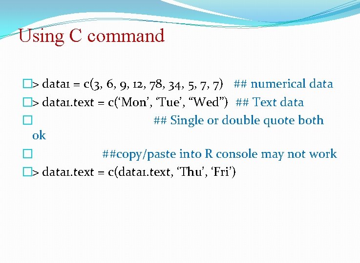
Using C command �> data 1 = c(3, 6, 9, 12, 78, 34, 5, 7, 7) ## numerical data �> data 1. text = c(‘Mon’, ‘Tue’, “Wed”) ## Text data � ## Single or double quote both ok � ##copy/paste into R console may not work �> data 1. text = c(data 1. text, ‘Thu’, ‘Fri’)

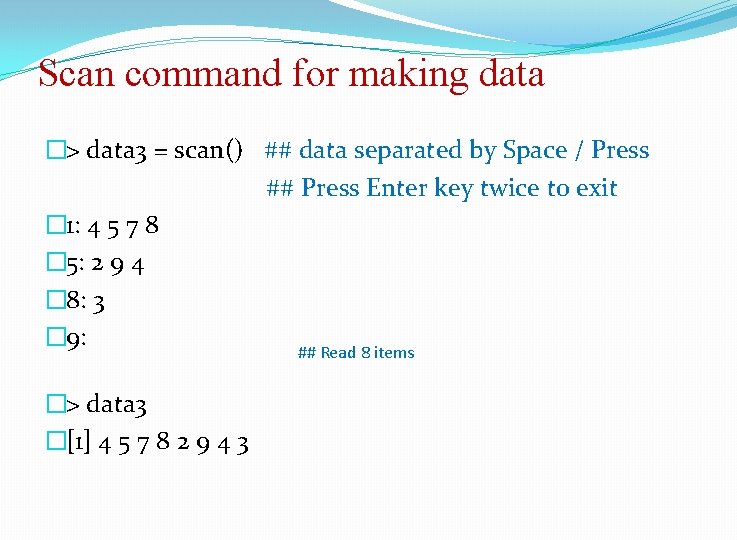
Scan command for making data �> data 3 = scan() ## data separated by Space / Press ## Press Enter key twice to exit � 1: 4 5 7 8 � 5: 2 9 4 � 8: 3 � 9: ## Read 8 items �> data 3 �[1] 4 5 7 8 2 9 4 3

Scan command for making data � > d 3 = scan(what = ‘character’) � 1: mon � 2: tue � 3: wed thu � 5: � > d 3 � [1] "mon" "tue" "wed" "thu" � > d 3[2] � [1] "tue" � � > d 3[2]='mon' � � > d 3 � [1] "mon" "wed" "thu" �> d 3[6]='sat' � �> d 3 �[1] "mon" "wed" "thu" NA "sat" � �> d 3[2]='tue' � �> d 3[5] = 'fri' � �> d 3 �[1] "mon" "tue" "wed" "thu" "fri" "sat"

Concept of working directory �>getwd() �[1] "C: UsersDSamantaRDatabase" � �> setwd('D: Data AnalyticsProjectDatabase) � �> dir() ## working directory listing � �>ls() ## Workspace listing of objects � �>rm(‘object’) ## Remove an element “object”, if exist � �> rm(list = ls()) ## Cleaning

Reading data from a data file � � � � � > setwd("D: /arpita/data analytics/my work") #Set the working directory to file location > getwd() [1] "D: /arpita/data analytics/my work“ > dir() [1] "Arv. txt" "Dining. At. SFO" "Latent. View-DPL" "TC-10 -Rec. csv" "TC. csv" rm(list=ls(all=TRUE)) # Refresh session > data=read. csv('iris. csv', header = T, sep=", ") (data = read. table(‘iris. csv', header = T, sep = ', ')) > ls() [1] "data" > str(data) 'data. frame': 149 obs. of 5 variables: $ X 5. 1 : num 4. 9 4. 7 4. 6 5 5. 4 4. 6 5 4. 4 4. 9 5. 4. . . $ X 3. 5 : num 3 3. 2 3. 1 3. 6 3. 9 3. 4 2. 9 3. 1 3. 7. . . $ X 1. 4 : num 1. 4 1. 3 1. 5 1. 4 1. 7 1. 4 1. 5. . . $ X 0. 2 : num 0. 2 0. 4 0. 3 0. 2 0. 1 0. 2. . . $ Iris. setosa: Factor w/ 3 levels "Iris-setosa", . . : 1 1 1 1 1. . .

Accessing elements from a file � > data$X 5. 1 � [1] 4. 9 4. 7 4. 6 5. 0 5. 4 4. 6 5. 0 4. 4 4. 9 5. 4 4. 8 4. 3 5. 8 5. 7 � > data$X 5. 1[7]=5. 2 � > data$X 5. 1 � [1] 4. 9 4. 7 4. 6 5. 0 5. 4 4. 6 5. 2 4. 4 4. 9 5. 4 4. 8 4. 3 5. 8 5. 7 #Note: This change has happened in workspace only not in the file. � How to make it permanent? � write. csv / write. table � >write. table(data, file =‘iris_mod. csv', row. names = FALSE, sep = ', ') � If row. names is TRUE, R adds one ID column in the beginning of file. � So its suggested to use row. names = FALSE option � >write. csv(data, file ==‘iris_mod. csv', row. names = TRUE) ## to test

Different data items in R �Vector �Matrix �Data Frame �List

Vectors in R �>x=c(1, 2, 3, 4, 56) �>x �> x[2] �> x = c(3, 4, NA, 5) �>mean(x) �[1] NA �>mean(x, rm. NA=T) �[1] 4 �> x = c(3, 4, NULL, 5) �>mean(x) �[1] 4

More on Vectors in R � >y = c(x, c(-1, 5), x) � >length(y) � There are useful methods to create long vectors whose elements are in arithmetic progression: � > x=1: 20 �>x � � If the common difference is not 1 or -1 then we can use the seq function � > y=seq(2, 5, 0. 3) �>y � [1] 2. 0 2. 3 2. 6 2. 9 3. 2 3. 5 3. 8 4. 1 4. 4 4. 7 5. 0 � > length(y) � [1] 11

More on Vectors in R � > x=1: 5 � > mean(x) � [1] 3 �> x � [1] 1 2 3 4 5 � > x^2 � [1] 1 4 9 16 25 � > x+1 � [1] 2 3 4 5 6 � > 2*x � [1] 2 4 6 8 10 � > exp(sqrt(x)) � [1] 2. 718282 4. 113250 5. 652234 7. 389056 9. 356469 � It is very easy to add/subtract/multiply/divide two vectors entry by entry. � > y=c(0, 3, 4, 0) � > x+y � [1] 1 5 7 4 5 � > y=c(0, 3, 4, 0, 9) � > x+y � [1] 1 5 7 4 14 � Warning message: � In x + y : longer object length is not a multiple of shorter object length � > x=1: 6 � > y=c(9, 8) � > x+y � [1] 10 10 12 12 14 14

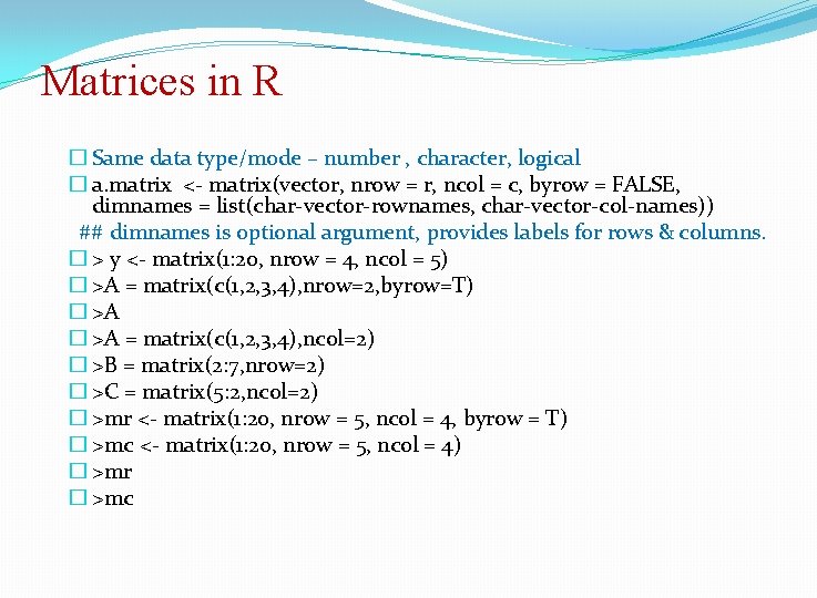
Matrices in R � Same data type/mode – number , character, logical � a. matrix <- matrix(vector, nrow = r, ncol = c, byrow = FALSE, dimnames = list(char-vector-rownames, char-vector-col-names)) ## dimnames is optional argument, provides labels for rows & columns. � > y <- matrix(1: 20, nrow = 4, ncol = 5) � >A = matrix(c(1, 2, 3, 4), nrow=2, byrow=T) � >A = matrix(c(1, 2, 3, 4), ncol=2) � >B = matrix(2: 7, nrow=2) � >C = matrix(5: 2, ncol=2) � >mr <- matrix(1: 20, nrow = 5, ncol = 4, byrow = T) � >mc <- matrix(1: 20, nrow = 5, ncol = 4) � >mr � >mc

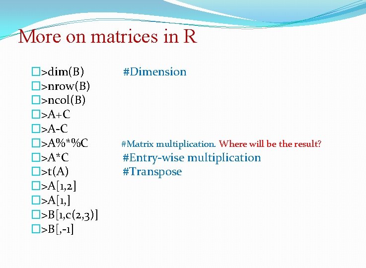
More on matrices in R �>dim(B) �>nrow(B) �>ncol(B) �>A+C �>A-C �>A%*%C �>A*C �>t(A) �>A[1, 2] �>A[1, ] �>B[1, c(2, 3)] �>B[, -1] #Dimension #Matrix multiplication. Where will be the result? #Entry-wise multiplication #Transpose

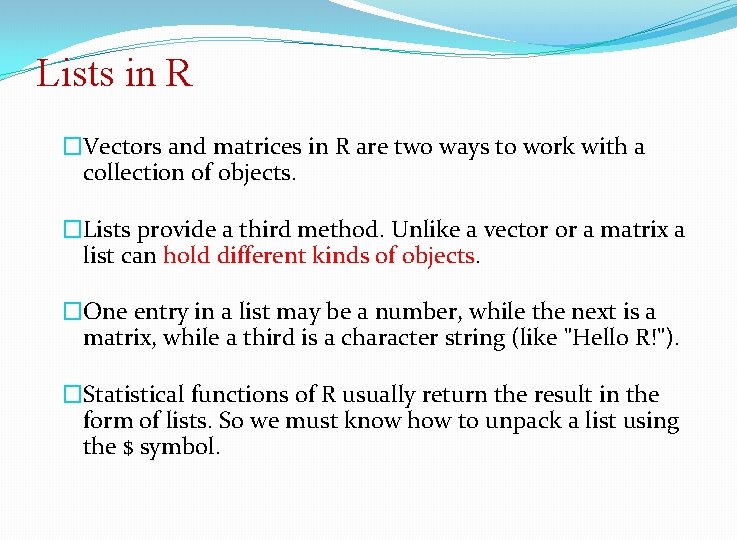
Lists in R �Vectors and matrices in R are two ways to work with a collection of objects. �Lists provide a third method. Unlike a vector or a matrix a list can hold different kinds of objects. �One entry in a list may be a number, while the next is a matrix, while a third is a character string (like "Hello R!"). �Statistical functions of R usually return the result in the form of lists. So we must know how to unpack a list using the $ symbol.

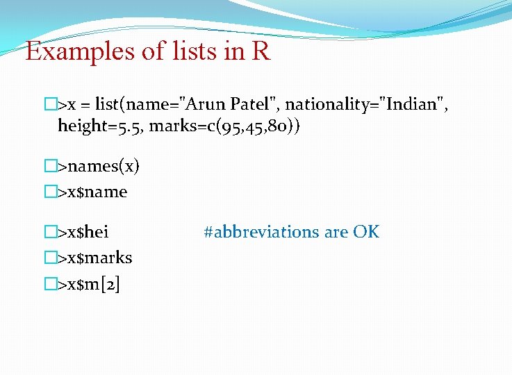
Examples of lists in R �>x = list(name="Arun Patel", nationality="Indian", height=5. 5, marks=c(95, 45, 80)) �>names(x) �>x$name �>x$hei �>x$marks �>x$m[2] #abbreviations are OK

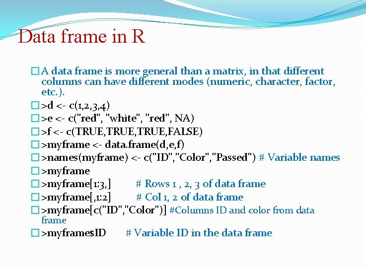
Data frame in R �A data frame is more general than a matrix, in that different columns can have different modes (numeric, character, factor, etc. ). �>d <- c(1, 2, 3, 4) �>e <- c("red", "white", "red", NA) �>f <- c(TRUE, FALSE) �>myframe <- data. frame(d, e, f) �>names(myframe) <- c("ID", "Color", "Passed") # Variable names �>myframe[1: 3, ] # Rows 1 , 2, 3 of data frame �>myframe[, 1: 2] # Col 1, 2 of data frame �>myframe[c("ID", "Color")] #Columns ID and color from data frame �>myframe$ID # Variable ID in the data frame

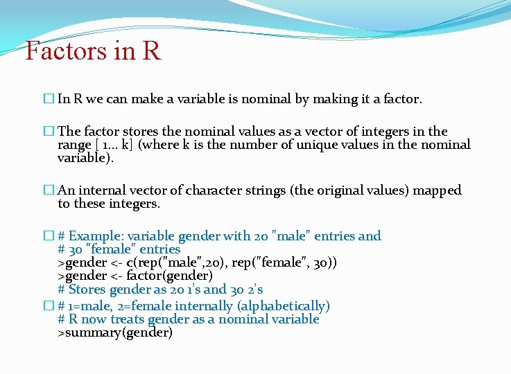
Factors in R � In R we can make a variable is nominal by making it a factor. � The factor stores the nominal values as a vector of integers in the range [ 1. . . k] (where k is the number of unique values in the nominal variable). � An internal vector of character strings (the original values) mapped to these integers. � # Example: variable gender with 20 "male" entries and # 30 "female" entries >gender <- c(rep("male", 20), rep("female", 30)) >gender <- factor(gender) # Stores gender as 20 1’s and 30 2’s � # 1=male, 2=female internally (alphabetically) # R now treats gender as a nominal variable >summary(gender)

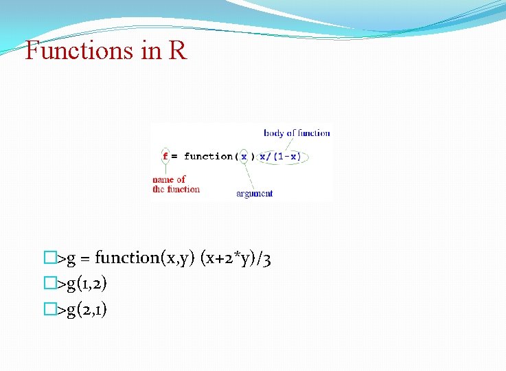
Functions in R �>g = function(x, y) (x+2*y)/3 �>g(1, 2) �>g(2, 1)

Any question? You may post your question(s) at the “Discussion Forum” maintained in the course Web page! CS 40003: Data Analytics 33

Just a minute to mark your attendance CS 40003: Data Analytics 34