CS 3343 Analysis of Algorithms Lecture 21 Introduction

- Slides: 56

CS 3343: Analysis of Algorithms Lecture 21: Introduction to Graphs

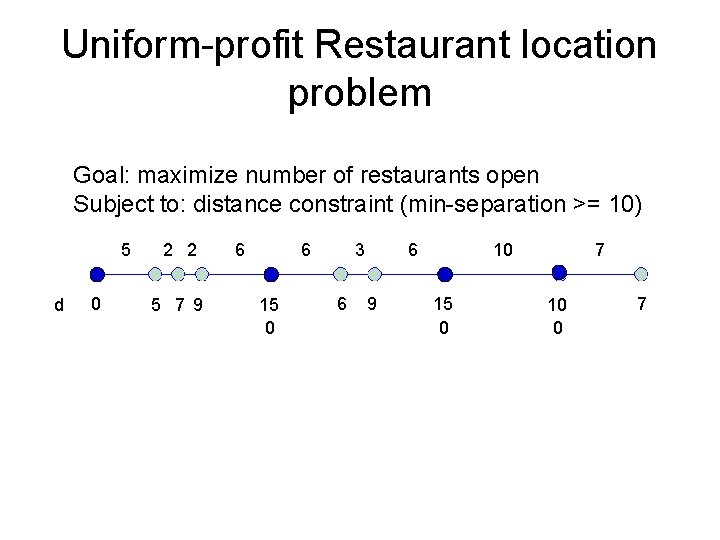
Uniform-profit Restaurant location problem Goal: maximize number of restaurants open Subject to: distance constraint (min-separation >= 10) 5 d 0 2 2 5 7 9 6 6 15 0 3 6 6 9 10 15 0 7 10 0 7

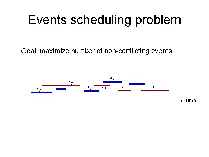
Events scheduling problem Goal: maximize number of non-conflicting events e 3 e 1 e 2 e 6 e 4 e 5 e 8 e 7 e 9 Time

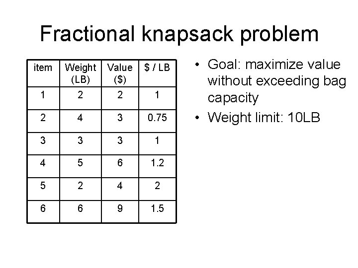
Fractional knapsack problem item Weight (LB) Value ($) $ / LB 1 2 2 1 2 4 3 0. 75 3 3 3 1 4 5 6 1. 2 5 2 4 2 6 6 9 1. 5 • Goal: maximize value without exceeding bag capacity • Weight limit: 10 LB

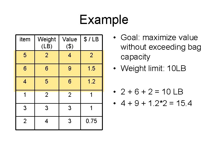
Example item Weight (LB) Value ($) $ / LB 5 2 4 2 6 6 9 1. 5 4 5 6 1. 2 1 2 2 1 3 3 3 1 2 4 3 0. 75 • Goal: maximize value without exceeding bag capacity • Weight limit: 10 LB • 2 + 6 + 2 = 10 LB • 4 + 9 + 1. 2*2 = 15. 4

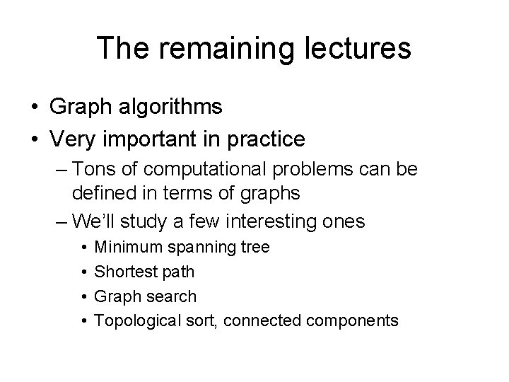
The remaining lectures • Graph algorithms • Very important in practice – Tons of computational problems can be defined in terms of graphs – We’ll study a few interesting ones • • Minimum spanning tree Shortest path Graph search Topological sort, connected components

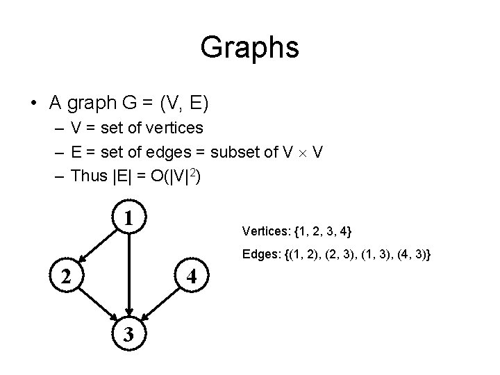
Graphs • A graph G = (V, E) – V = set of vertices – E = set of edges = subset of V V – Thus |E| = O(|V|2) 1 Vertices: {1, 2, 3, 4} Edges: {(1, 2), (2, 3), (1, 3), (4, 3)} 2 4 3

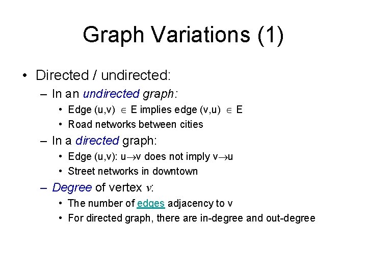
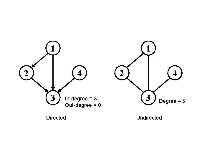
Graph Variations (1) • Directed / undirected: – In an undirected graph: • Edge (u, v) E implies edge (v, u) E • Road networks between cities – In a directed graph: • Edge (u, v): u v does not imply v u • Street networks in downtown – Degree of vertex v: • The number of edges adjacency to v • For directed graph, there are in-degree and out-degree

1 1 2 4 3 In-degree = 3 Out-degree = 0 Directed 2 4 3 Degree = 3 Undirected

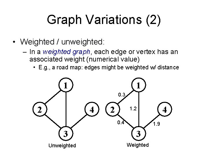
Graph Variations (2) • Weighted / unweighted: – In a weighted graph, each edge or vertex has an associated weight (numerical value) • E. g. , a road map: edges might be weighted w/ distance 1 1 0. 3 2 4 2 0. 4 3 Unweighted 4 1. 2 1. 9 3 Weighted

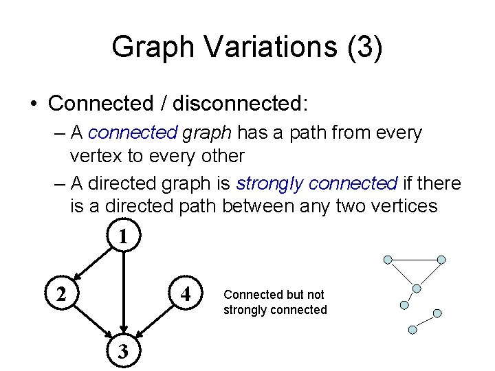
Graph Variations (3) • Connected / disconnected: – A connected graph has a path from every vertex to every other – A directed graph is strongly connected if there is a directed path between any two vertices 1 2 4 3 Connected but not strongly connected

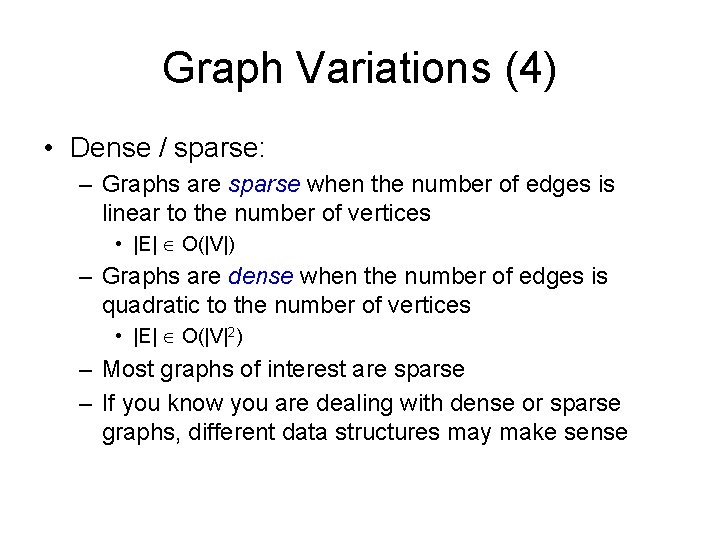
Graph Variations (4) • Dense / sparse: – Graphs are sparse when the number of edges is linear to the number of vertices • |E| O(|V|) – Graphs are dense when the number of edges is quadratic to the number of vertices • |E| O(|V|2) – Most graphs of interest are sparse – If you know you are dealing with dense or sparse graphs, different data structures may make sense

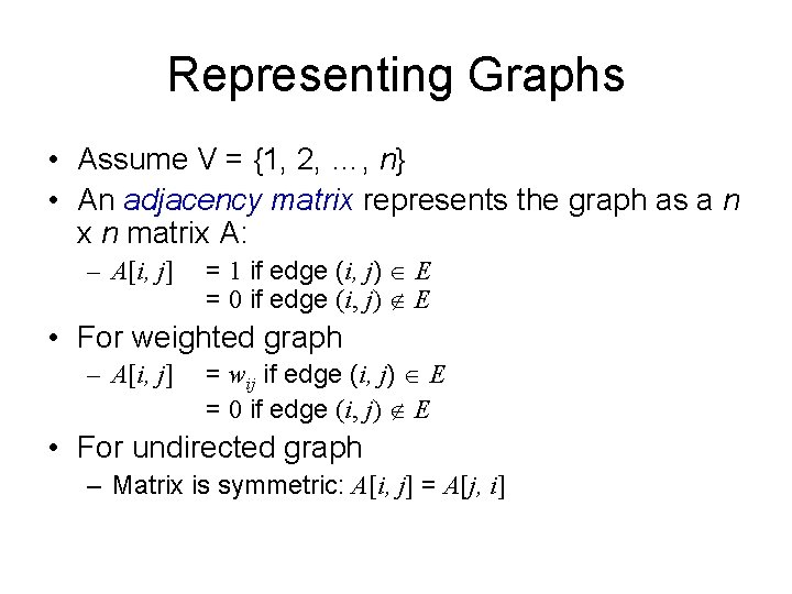
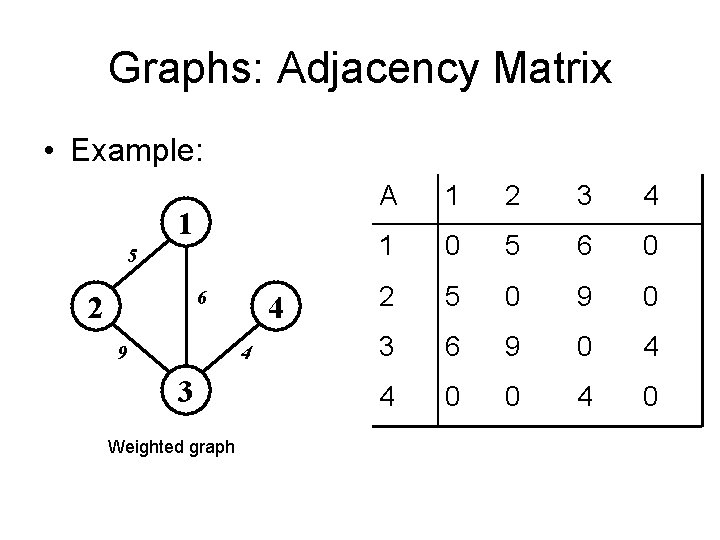
Representing Graphs • Assume V = {1, 2, …, n} • An adjacency matrix represents the graph as a n x n matrix A: – A[i, j] = 1 if edge (i, j) E = 0 if edge (i, j) E • For weighted graph – A[i, j] = wij if edge (i, j) E = 0 if edge (i, j) E • For undirected graph – Matrix is symmetric: A[i, j] = A[j, i]

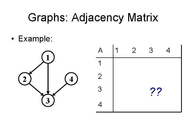
Graphs: Adjacency Matrix • Example: A 1 2 2 3 1 4 2 3 3 1 4 ? ? 4

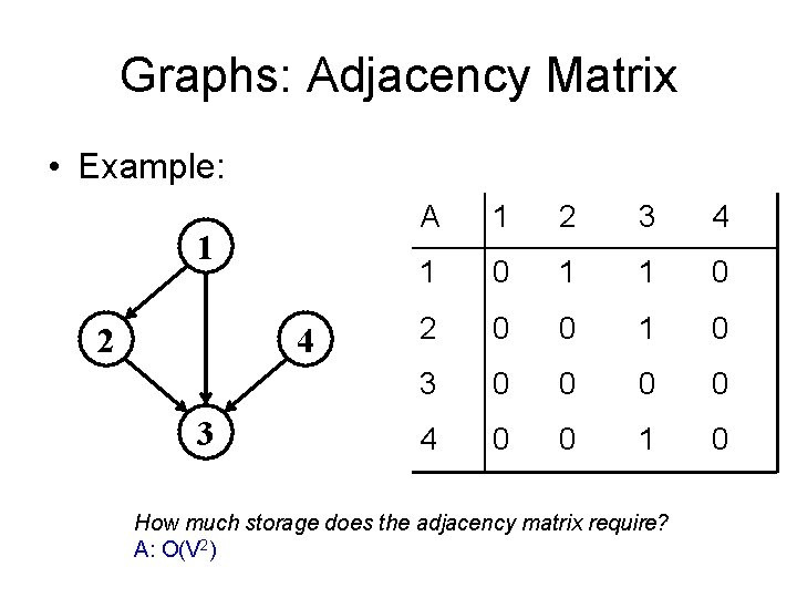
Graphs: Adjacency Matrix • Example: 1 2 4 3 A 1 2 3 4 1 0 1 1 0 2 0 0 1 0 3 0 0 4 0 0 1 0 How much storage does the adjacency matrix require? A: O(V 2)

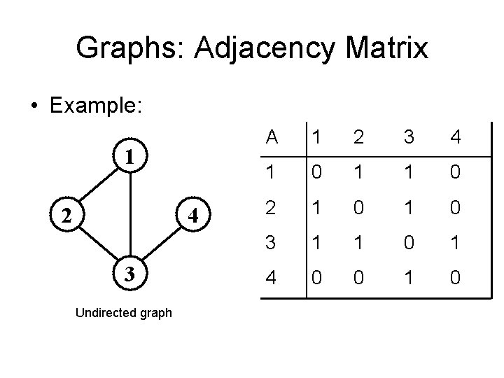
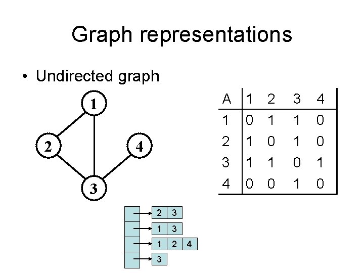
Graphs: Adjacency Matrix • Example: 1 2 4 3 Undirected graph A 1 2 3 4 1 0 1 1 0 2 1 0 3 1 1 0 1 4 0 0 1 0

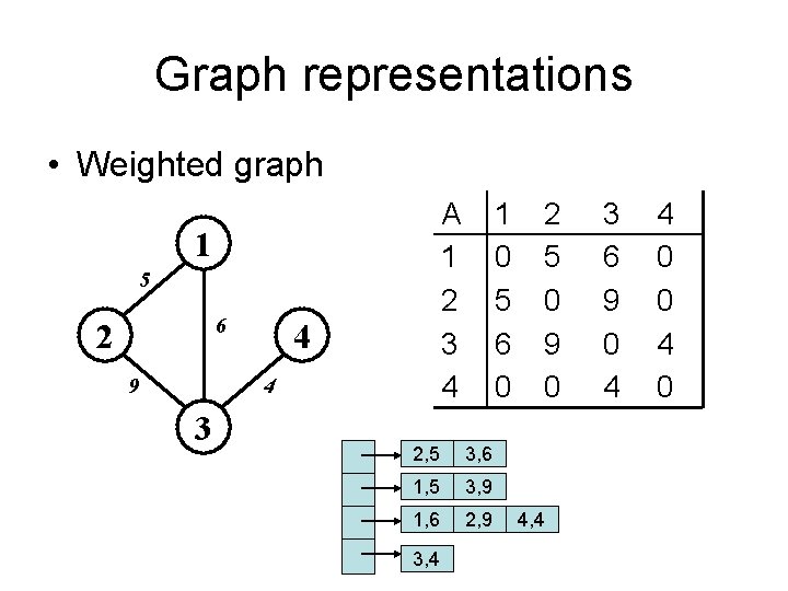
Graphs: Adjacency Matrix • Example: 1 5 6 2 9 4 4 3 Weighted graph A 1 2 3 4 1 0 5 6 0 2 5 0 9 0 3 6 9 0 4 4 0 0 4 0

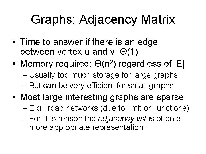
Graphs: Adjacency Matrix • Time to answer if there is an edge between vertex u and v: Θ(1) • Memory required: Θ(n 2) regardless of |E| – Usually too much storage for large graphs – But can be very efficient for small graphs • Most large interesting graphs are sparse – E. g. , road networks (due to limit on junctions) – For this reason the adjacency list is often a more appropriate representation

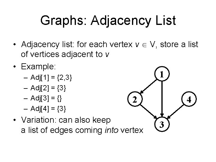
Graphs: Adjacency List • Adjacency list: for each vertex v V, store a list of vertices adjacent to v • Example: – – Adj[1] = {2, 3} Adj[2] = {3} Adj[3] = {} Adj[4] = {3} 1 2 • Variation: can also keep a list of edges coming into vertex 4 3

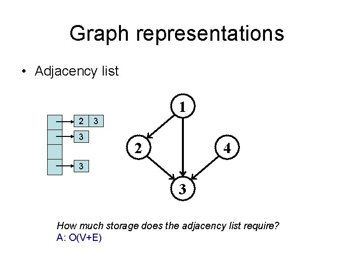
Graph representations • Adjacency list 1 2 3 3 2 4 3 3 How much storage does the adjacency list require? A: O(V+E)

Graph representations • Undirected graph 1 2 4 3 2 3 1 2 3 4 A 1 2 0 1 1 0 3 1 1 4 0 0 3 4 1 1 0 0 0 1 1 0

Graph representations • Weighted graph A 1 2 3 4 1 5 6 2 9 4 4 3 1 0 5 6 0 2, 5 3, 6 1, 5 3, 9 1, 6 2, 9 3, 4 2 5 0 9 0 4, 4 3 6 9 0 4 4 0 0 4 0

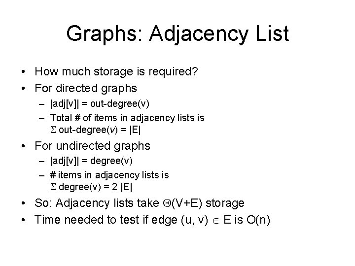
Graphs: Adjacency List • How much storage is required? • For directed graphs – |adj[v]| = out-degree(v) – Total # of items in adjacency lists is out-degree(v) = |E| • For undirected graphs – |adj[v]| = degree(v) – # items in adjacency lists is degree(v) = 2 |E| • So: Adjacency lists take (V+E) storage • Time needed to test if edge (u, v) E is O(n)

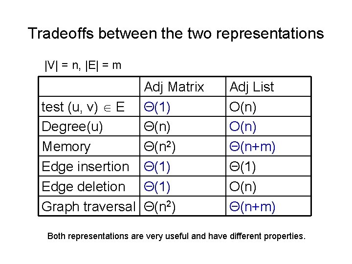
Tradeoffs between the two representations |V| = n, |E| = m Adj Matrix test (u, v) E Θ(1) Degree(u) Θ(n) Memory Θ(n 2) Edge insertion Θ(1) Edge deletion Θ(1) Graph traversal Θ(n 2) Adj List O(n) Θ(n+m) Θ(1) O(n) Θ(n+m) Both representations are very useful and have different properties.

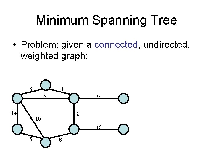
Minimum Spanning Tree • Problem: given a connected, undirected, weighted graph: 6 4 5 14 9 2 10 15 3 8

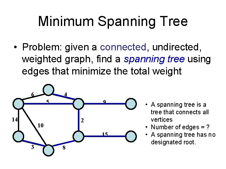
Minimum Spanning Tree • Problem: given a connected, undirected, weighted graph, find a spanning tree using edges that minimize the total weight 6 4 5 14 9 2 10 15 3 8 • A spanning tree is a tree that connects all vertices • Number of edges = ? • A spanning tree has no designated root.

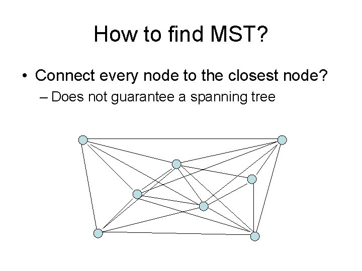
How to find MST? • Connect every node to the closest node? – Does not guarantee a spanning tree

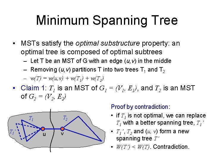
Minimum Spanning Tree • MSTs satisfy the optimal substructure property: an optimal tree is composed of optimal subtrees – Let T be an MST of G with an edge (u, v) in the middle – Removing (u, v) partitions T into two trees T 1 and T 2 – w(T) = w(u, v) + w(T 1) + w(T 2) • Claim 1: T 1 is an MST of G 1 = (V 1, E 1), and T 2 is an MST of G 2 = (V 2, E 2) T 2 T 1 ’ u v Proof by contradiction: • if T 1 is not optimal, we can replace T 1 with a better spanning tree, T 1’ • T 1’, T 2 and (u, v) form a new spanning tree T’ • W(T’) < W(T). Contradiction.

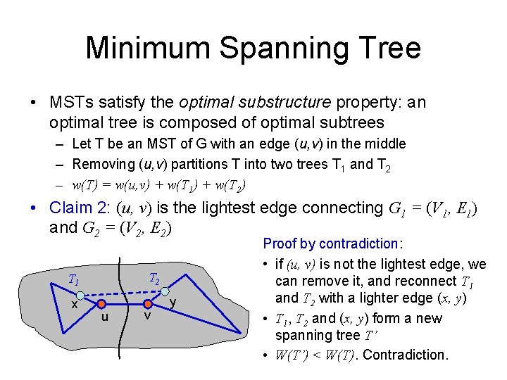
Minimum Spanning Tree • MSTs satisfy the optimal substructure property: an optimal tree is composed of optimal subtrees – Let T be an MST of G with an edge (u, v) in the middle – Removing (u, v) partitions T into two trees T 1 and T 2 – w(T) = w(u, v) + w(T 1) + w(T 2) • Claim 2: (u, v) is the lightest edge connecting G 1 = (V 1, E 1) and G 2 = (V 2, E 2) T 2 T 1 x u v y Proof by contradiction: • if (u, v) is not the lightest edge, we can remove it, and reconnect T 1 and T 2 with a lighter edge (x, y) • T 1, T 2 and (x, y) form a new spanning tree T’ • W(T’) < W(T). Contradiction.

Algorithms • Generic idea: – Compute MSTs for sub-graphs – Connect two MSTs for sub-graphs with the lightest edge • Two of the most well-known algorithms – Prim’s algorithm – Kruskal’s algorithm – Let’s first talk about the ideas behind the algorithms without worrying about the implementation and analysis

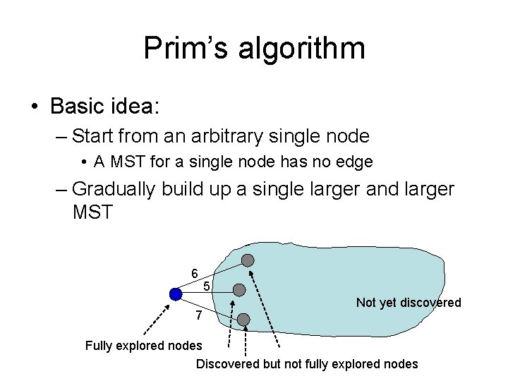
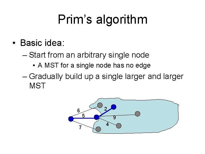
Prim’s algorithm • Basic idea: – Start from an arbitrary single node • A MST for a single node has no edge – Gradually build up a single larger and larger MST 6 7 5 Not yet discovered Fully explored nodes Discovered but not fully explored nodes

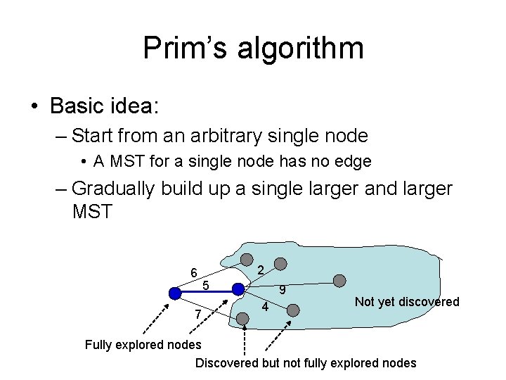
Prim’s algorithm • Basic idea: – Start from an arbitrary single node • A MST for a single node has no edge – Gradually build up a single larger and larger MST 6 7 2 5 9 4 Not yet discovered Fully explored nodes Discovered but not fully explored nodes

Prim’s algorithm • Basic idea: – Start from an arbitrary single node • A MST for a single node has no edge – Gradually build up a single larger and larger MST 6 7 2 5 9 4

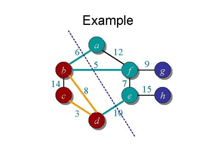
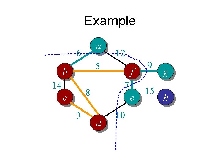
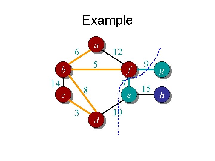
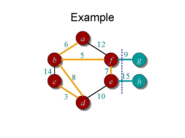
Prim’s algorithm in words • Randomly pick a vertex as the initial tree T • Gradually expand into a MST: – For each vertex that is not in T but directly connected to some nodes in T • Compute its minimum distance to any vertex in T – Select the vertex that is closest to T • Add it to T

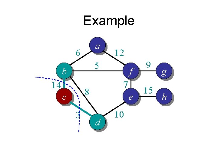
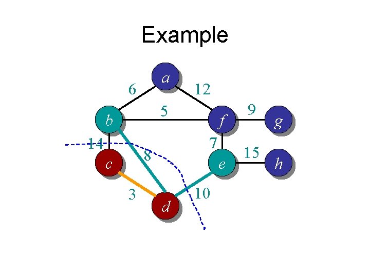
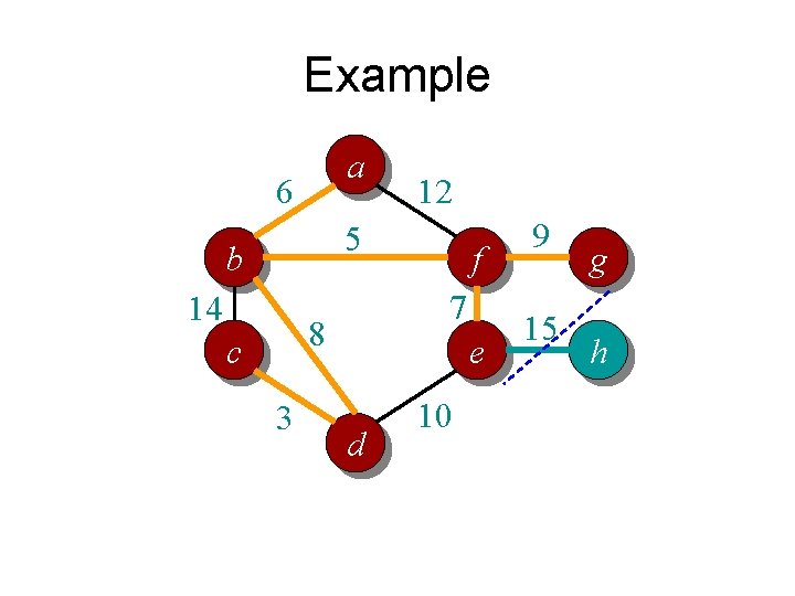
Example a 6 12 5 b 14 7 8 c 3 f e d 10 9 15 g h

Example a 6 12 5 b 14 7 8 c 3 f e d 10 9 15 g h

Example a 6 12 5 b 14 7 8 c 3 f e d 10 9 15 g h

Example a 6 12 5 b 14 7 8 c 3 f e d 10 9 15 g h

Example a 6 12 5 b 14 7 8 c 3 f e d 10 9 15 g h

Example a 6 12 5 b 14 7 8 c 3 f e d 10 9 15 g h

Example a 6 12 5 b 14 7 8 c 3 f e d 10 9 15 g h

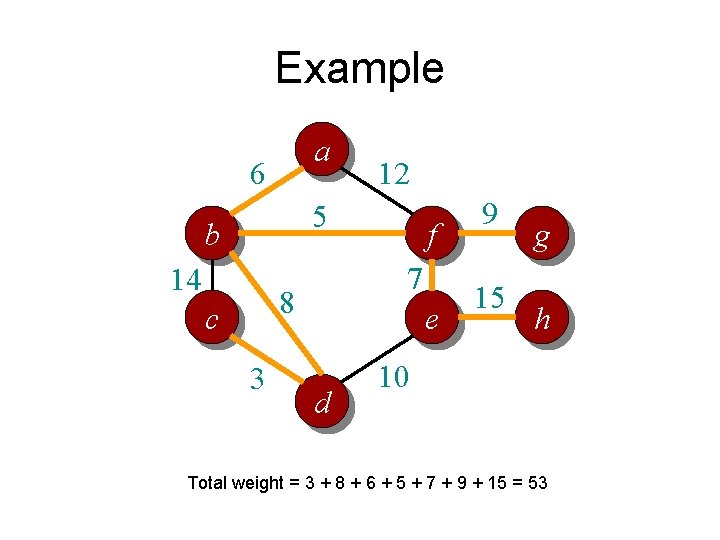
Example a 6 12 5 b 14 7 8 c 3 f e d 9 15 g h 10 Total weight = 3 + 8 + 6 + 5 + 7 + 9 + 15 = 53

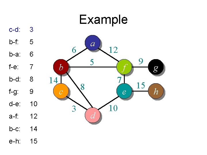
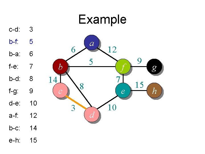
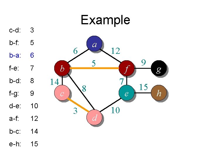
Kruskal’s algorithm • Basic idea: – Grow many small trees – Find two trees that are closest (i. e. , connected with the lightest edge), join them with the lightest edge – Terminate when a single tree forms

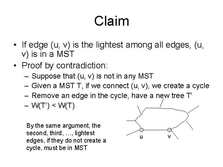
Claim • If edge (u, v) is the lightest among all edges, (u, v) is in a MST • Proof by contradiction: – – Suppose that (u, v) is not in any MST Given a MST T, if we connect (u, v), we create a cycle Remove an edge in the cycle, have a new tree T’ W(T’) < W(T) By the same argument, the second, third, …, lightest edges, if they do not create a cycle, must be in MST u v

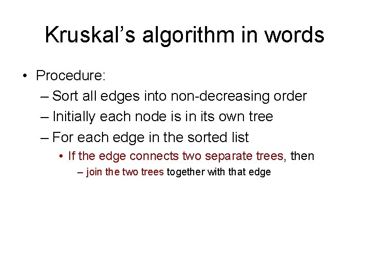
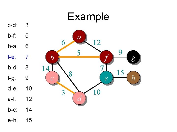
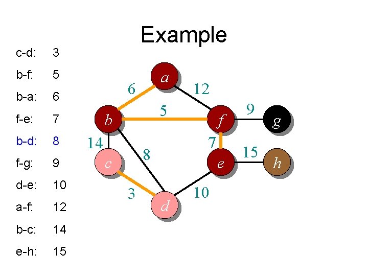
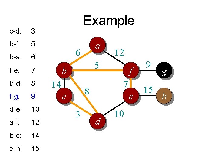
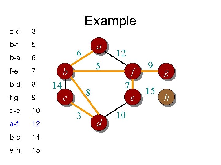
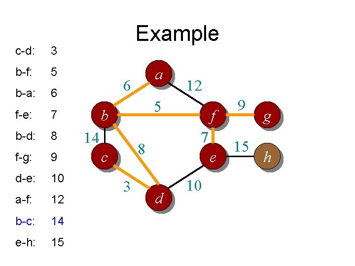
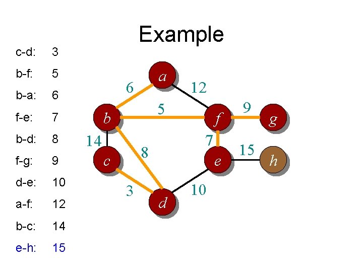
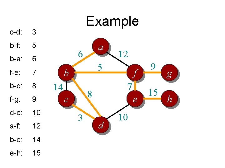
Kruskal’s algorithm in words • Procedure: – Sort all edges into non-decreasing order – Initially each node is in its own tree – For each edge in the sorted list • If the edge connects two separate trees, then – join the two trees together with that edge

c-d: 3 b-f: 5 b-a: 6 f-e: 7 b-d: 8 f-g: 9 d-e: 10 a-f: 12 b-c: 14 e-h: 15 Example a 6 12 5 b 14 7 8 c 3 f e d 10 9 15 g h

c-d: 3 b-f: 5 b-a: 6 f-e: 7 b-d: 8 f-g: 9 d-e: 10 a-f: 12 b-c: 14 e-h: 15 Example a 6 12 5 b 14 7 8 c 3 f e d 10 9 15 g h

c-d: 3 b-f: 5 b-a: 6 f-e: 7 b-d: 8 f-g: 9 d-e: 10 a-f: 12 b-c: 14 e-h: 15 Example a 6 12 5 b 14 7 8 c 3 f e d 10 9 15 g h

c-d: 3 b-f: 5 b-a: 6 f-e: 7 b-d: 8 f-g: 9 d-e: 10 a-f: 12 b-c: 14 e-h: 15 Example a 6 12 5 b 14 7 8 c 3 f e d 10 9 15 g h

c-d: 3 b-f: 5 b-a: 6 f-e: 7 b-d: 8 f-g: 9 d-e: 10 a-f: 12 b-c: 14 e-h: 15 Example a 6 12 5 b 14 7 8 c 3 f e d 10 9 15 g h

c-d: 3 b-f: 5 b-a: 6 f-e: 7 b-d: 8 f-g: 9 d-e: 10 a-f: 12 b-c: 14 e-h: 15 Example a 6 12 5 b 14 7 8 c 3 f e d 10 9 15 g h

c-d: 3 b-f: 5 b-a: 6 f-e: 7 b-d: 8 f-g: 9 d-e: 10 a-f: 12 b-c: 14 e-h: 15 Example a 6 12 5 b 14 7 8 c 3 f e d 10 9 15 g h

c-d: 3 b-f: 5 b-a: 6 f-e: 7 b-d: 8 f-g: 9 d-e: 10 a-f: 12 b-c: 14 e-h: 15 Example a 6 12 5 b 14 7 8 c 3 f e d 10 9 15 g h

c-d: 3 b-f: 5 b-a: 6 f-e: 7 b-d: 8 f-g: 9 d-e: 10 a-f: 12 b-c: 14 e-h: 15 Example a 6 12 5 b 14 7 8 c 3 f e d 10 9 15 g h

c-d: 3 b-f: 5 b-a: 6 f-e: 7 b-d: 8 f-g: 9 d-e: 10 a-f: 12 b-c: 14 e-h: 15 Example a 6 12 5 b 14 7 8 c 3 f e d 10 9 15 g h

c-d: 3 b-f: 5 b-a: 6 f-e: 7 b-d: 8 f-g: 9 d-e: 10 a-f: 12 b-c: 14 e-h: 15 Example a 6 12 5 b 14 7 8 c 3 f e d 10 9 15 g h