CS 1674 Intro to Computer Vision Visual Recognition

CS 1674: Intro to Computer Vision Visual Recognition Prof. Adriana Kovashka University of Pittsburgh October 22, 2019

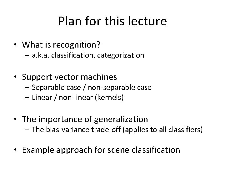
Plan for this lecture • What is recognition? – a. k. a. classification, categorization • Support vector machines – Separable case / non-separable case – Linear / non-linear (kernels) • The importance of generalization – The bias-variance trade-off (applies to all classifiers) • Example approach for scene classification

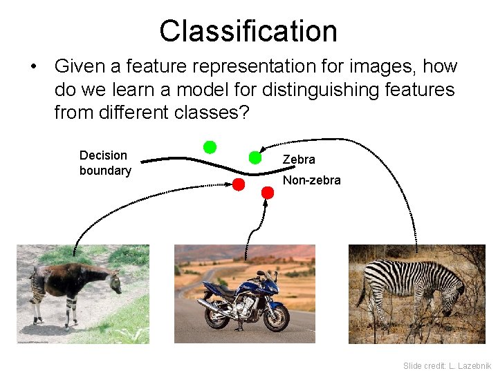
Classification • Given a feature representation for images, how do we learn a model for distinguishing features from different classes? Decision boundary Zebra Non-zebra Slide credit: L. Lazebnik

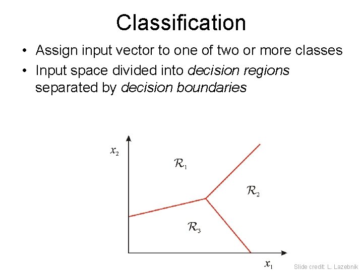
Classification • Assign input vector to one of two or more classes • Input space divided into decision regions separated by decision boundaries Slide credit: L. Lazebnik

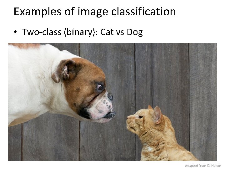
Examples of image classification • Two-class (binary): Cat vs Dog Adapted from D. Hoiem

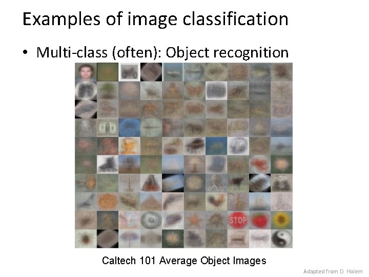
Examples of image classification • Multi-class (often): Object recognition Caltech 101 Average Object Images Adapted from D. Hoiem

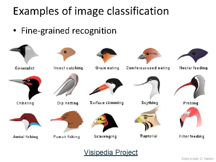
Examples of image classification • Fine-grained recognition Visipedia Project Slide credit: D. Hoiem

Examples of image classification • Place recognition Places Database [Zhou et al. NIPS 2014] Slide credit: D. Hoiem

Examples of image classification • Material recognition [Bell et al. CVPR 2015] Slide credit: D. Hoiem

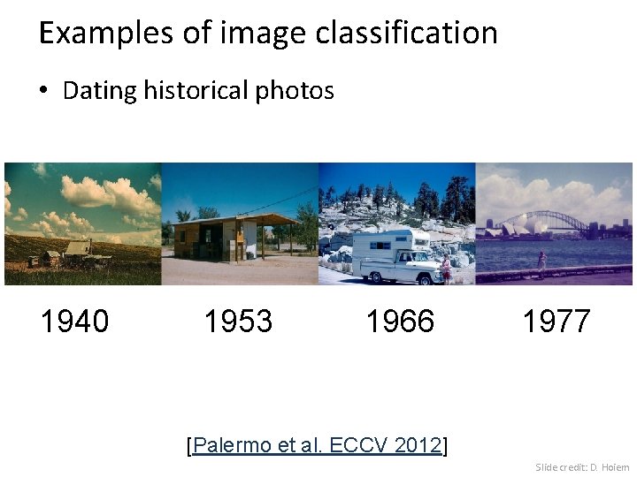
Examples of image classification • Dating historical photos 1940 1953 1966 1977 [Palermo et al. ECCV 2012] Slide credit: D. Hoiem

Examples of image classification • Image style recognition [Karayev et al. BMVC 2014] Slide credit: D. Hoiem

Recognition: A machine learning approach

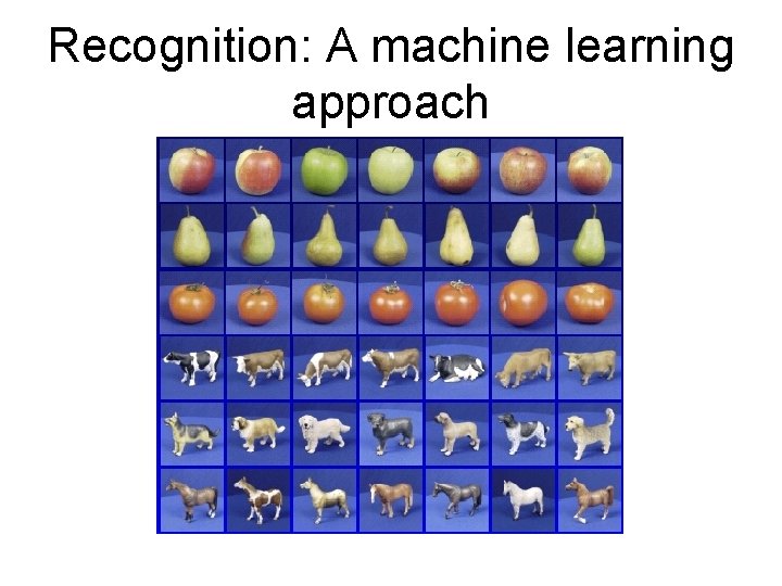
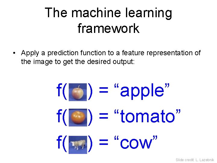
The machine learning framework • Apply a prediction function to a feature representation of the image to get the desired output: f( ) = “apple” f( ) = “tomato” f( ) = “cow” Slide credit: L. Lazebnik

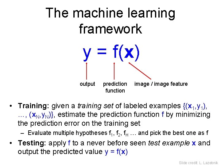
The machine learning framework y = f(x) output prediction function image / image feature • Training: given a training set of labeled examples {(x 1, y 1), …, (x. N, y. N)}, estimate the prediction function f by minimizing the prediction error on the training set – Evaluate multiple hypotheses f 1, f 2, f. H … and pick the best one as f • Testing: apply f to a never before seen test example x and output the predicted value y = f(x) Slide credit: L. Lazebnik

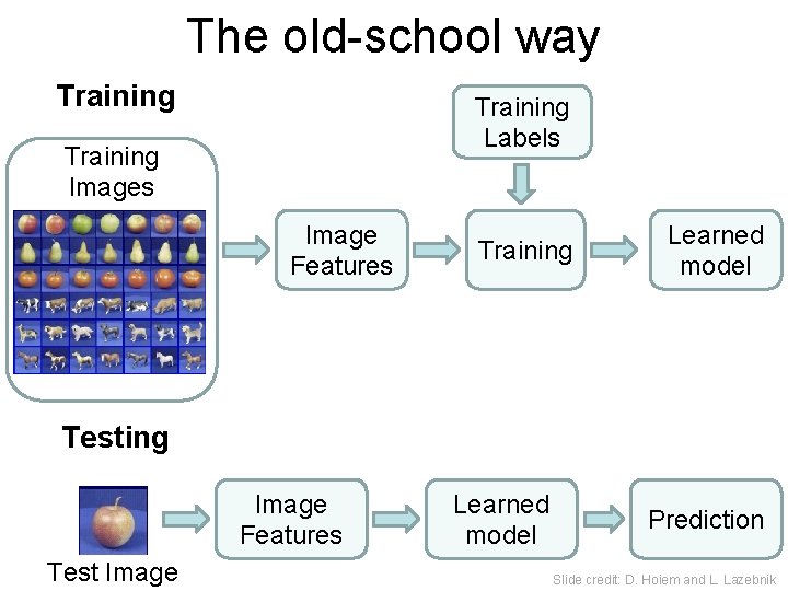
The old-school way Training Labels Training Images Image Features Training Learned model Testing Image Features Test Image Learned model Prediction Slide credit: D. Hoiem and L. Lazebnik

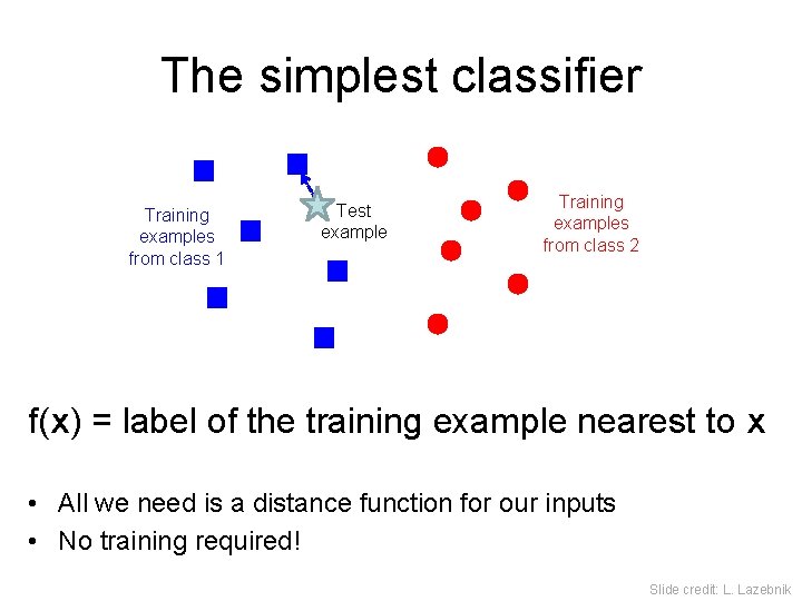
The simplest classifier Training examples from class 1 Test example Training examples from class 2 f(x) = label of the training example nearest to x • All we need is a distance function for our inputs • No training required! Slide credit: L. Lazebnik

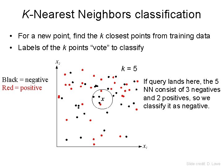
K-Nearest Neighbors classification • For a new point, find the k closest points from training data • Labels of the k points “vote” to classify k = 5 Black = negative Red = positive If query lands here, the 5 NN consist of 3 negatives and 2 positives, so we classify it as negative. Slide credit: D. Lowe

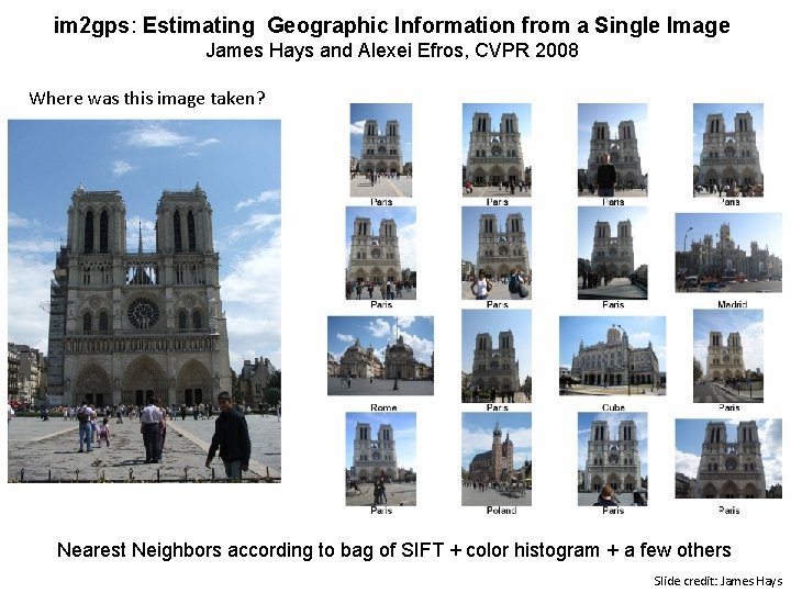
im 2 gps: Estimating Geographic Information from a Single Image James Hays and Alexei Efros, CVPR 2008 Where was this image taken? Nearest Neighbors according to bag of SIFT + color histogram + a few others Slide credit: James Hays

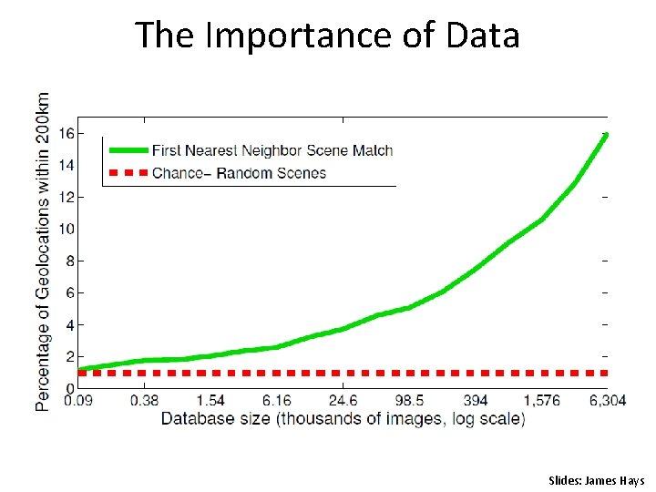
The Importance of Data Slides: James Hays

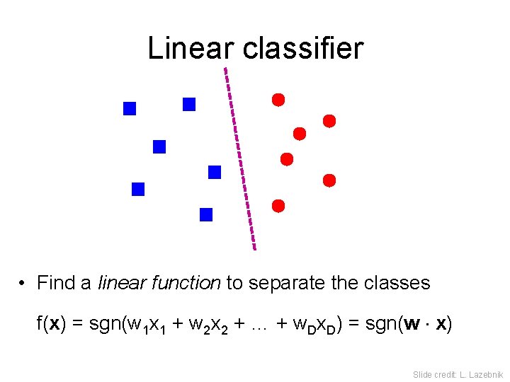
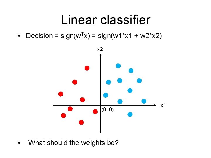
Linear classifier • Find a linear function to separate the classes f(x) = sgn(w 1 x 1 + w 2 x 2 + … + w. Dx. D) = sgn(w x) Slide credit: L. Lazebnik

Linear classifier • Decision = sign(w. Tx) = sign(w 1*x 1 + w 2*x 2) x 2 (0, 0) • What should the weights be? x 1

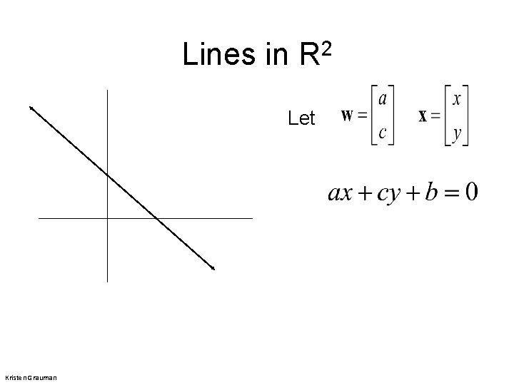
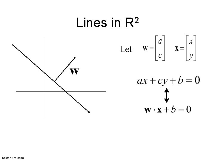
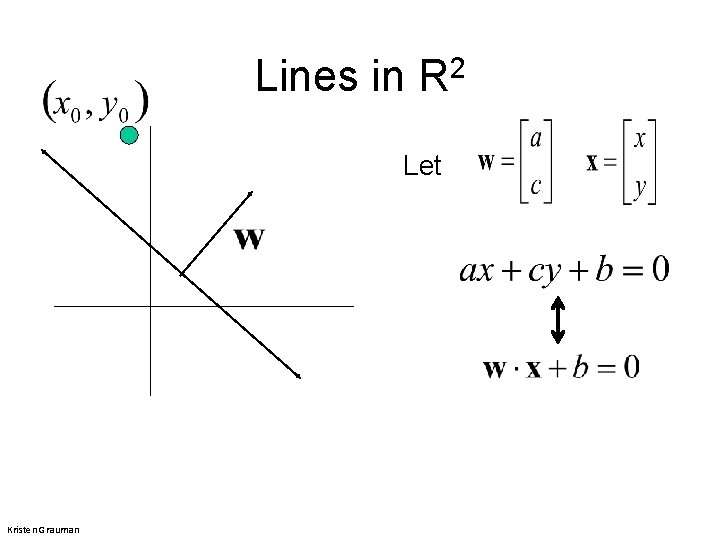
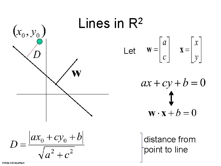
Lines in R 2 Let Kristen Grauman

Lines in R 2 Let Kristen Grauman

Lines in R 2 Let Kristen Grauman

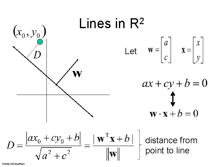
Lines in R 2 Let distance from point to line Kristen Grauman

Lines in R 2 Let distance from point to line Kristen Grauman

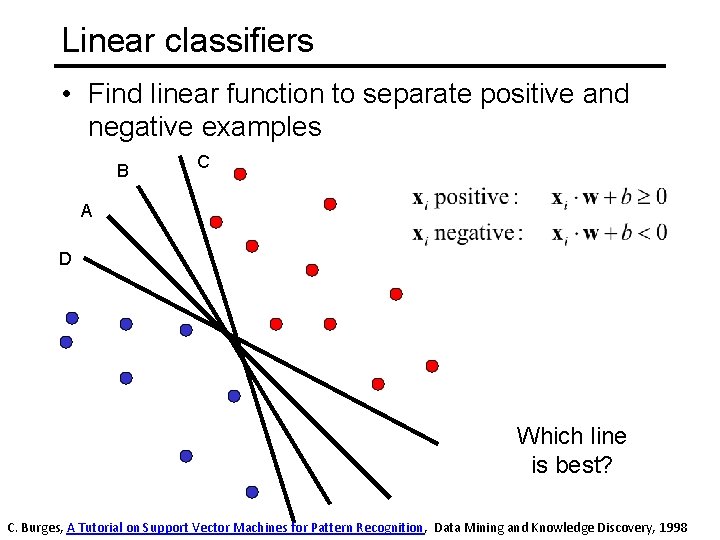
Linear classifiers • Find linear function to separate positive and negative examples B C A D Which line is best? C. Burges, A Tutorial on Support Vector Machines for Pattern Recognition, Data Mining and Knowledge Discovery, 1998

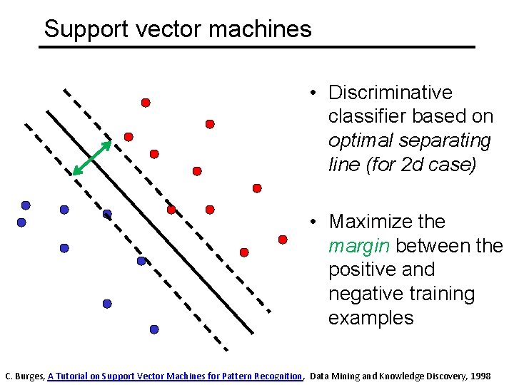
Support vector machines • Discriminative classifier based on optimal separating line (for 2 d case) • Maximize the margin between the positive and negative training examples C. Burges, A Tutorial on Support Vector Machines for Pattern Recognition, Data Mining and Knowledge Discovery, 1998

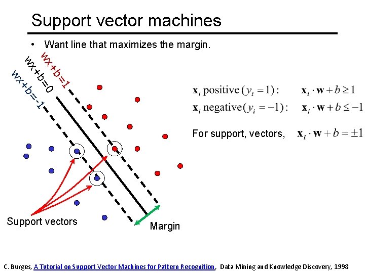
Support vector machines • Want line that maximizes the margin. =1 +b wx =0 1 +b wx +b= wx For support, vectors, Support vectors Margin C. Burges, A Tutorial on Support Vector Machines for Pattern Recognition, Data Mining and Knowledge Discovery, 1998

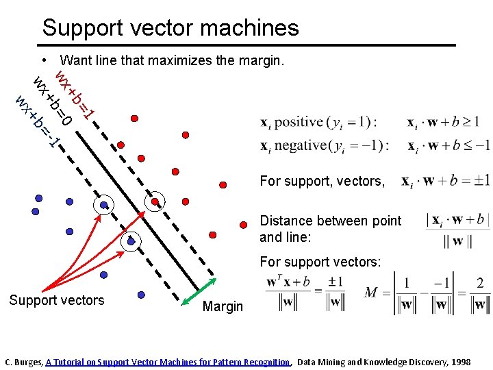
Support vector machines • Want line that maximizes the margin. =1 +b wx =0 1 +b wx +b= wx For support, vectors, Distance between point and line: For support vectors: Support vectors Margin C. Burges, A Tutorial on Support Vector Machines for Pattern Recognition, Data Mining and Knowledge Discovery, 1998

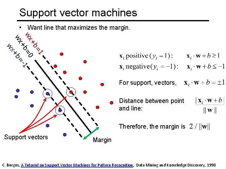
Support vector machines • Want line that maximizes the margin. =1 +b wx =0 1 +b wx +b= wx For support, vectors, Distance between point and line: Therefore, the margin is 2 Support vectors / ||w|| Margin C. Burges, A Tutorial on Support Vector Machines for Pattern Recognition, Data Mining and Knowledge Discovery, 1998

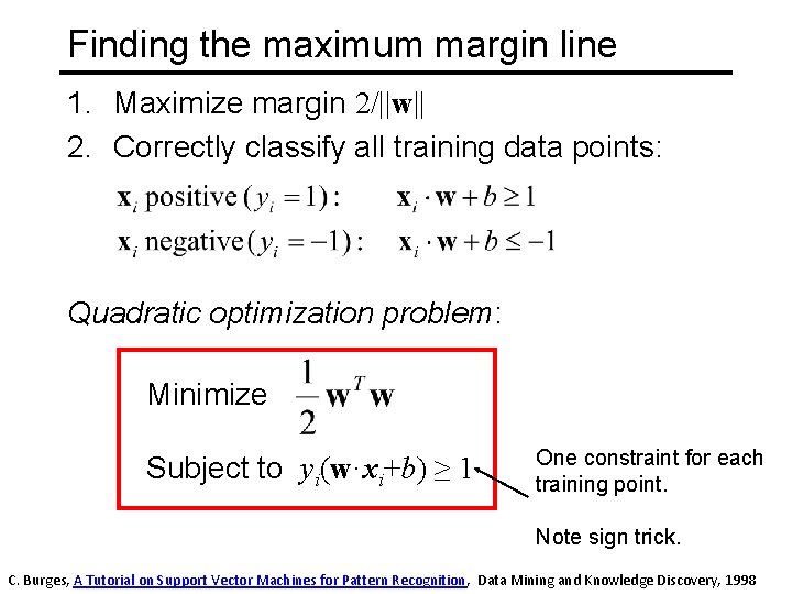
Finding the maximum margin line 1. Maximize margin 2/||w|| 2. Correctly classify all training data points: Quadratic optimization problem: Minimize Subject to yi(w·xi+b) ≥ 1 One constraint for each training point. Note sign trick. C. Burges, A Tutorial on Support Vector Machines for Pattern Recognition, Data Mining and Knowledge Discovery, 1998

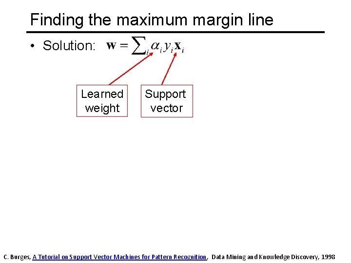
Finding the maximum margin line • Solution: Learned weight Support vector C. Burges, A Tutorial on Support Vector Machines for Pattern Recognition, Data Mining and Knowledge Discovery, 1998

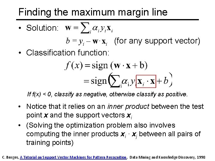
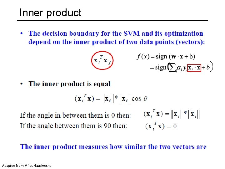
Finding the maximum margin line • Solution: b = yi – w·xi (for any support vector) • Classification function: If f(x) < 0, classify as negative, otherwise classify as positive. • Notice that it relies on an inner product between the test point x and the support vectors xi • (Solving the optimization problem also involves computing the inner products xi · xj between all pairs of training points) C. Burges, A Tutorial on Support Vector Machines for Pattern Recognition, Data Mining and Knowledge Discovery, 1998

Inner product Adapted from Milos Hauskrecht

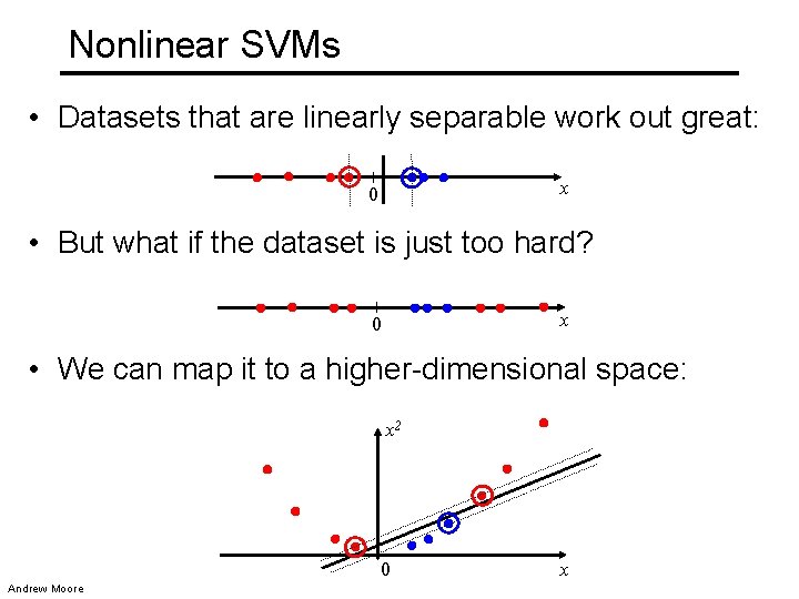
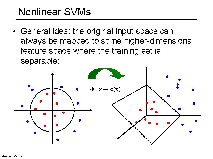
Nonlinear SVMs • Datasets that are linearly separable work out great: x 0 • But what if the dataset is just too hard? x 0 • We can map it to a higher-dimensional space: x 2 0 Andrew Moore x

Nonlinear SVMs • General idea: the original input space can always be mapped to some higher-dimensional feature space where the training set is separable: Φ: x → φ(x) Andrew Moore

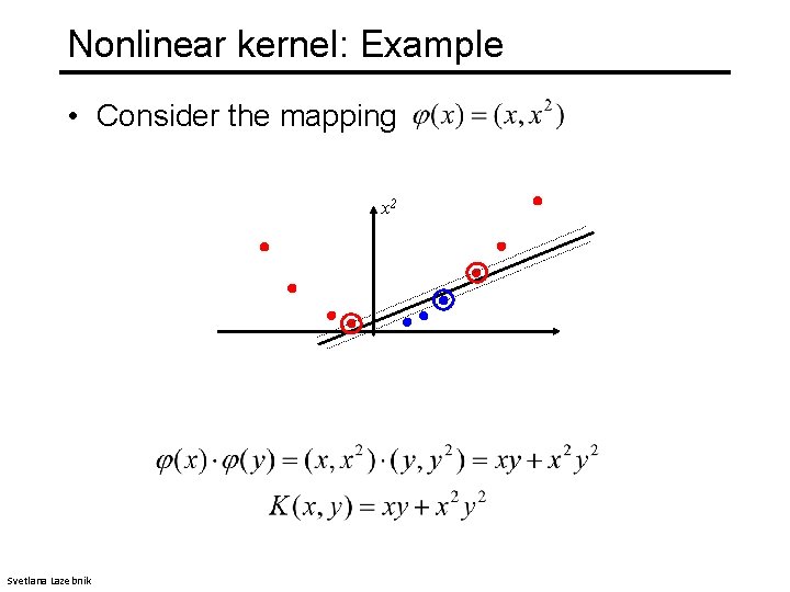
Nonlinear kernel: Example • Consider the mapping x 2 Svetlana Lazebnik

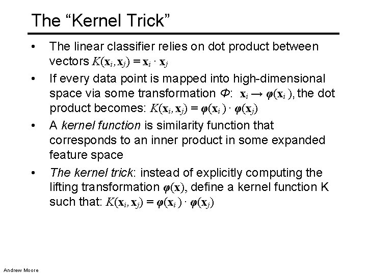
The “Kernel Trick” • • Andrew Moore The linear classifier relies on dot product between vectors K(xi , xj) = xi · xj If every data point is mapped into high-dimensional space via some transformation Φ: xi → φ(xi ), the dot product becomes: K(xi , xj) = φ(xi ) · φ(xj) A kernel function is similarity function that corresponds to an inner product in some expanded feature space The kernel trick: instead of explicitly computing the lifting transformation φ(x), define a kernel function K such that: K(xi , xj) = φ(xi ) · φ(xj)

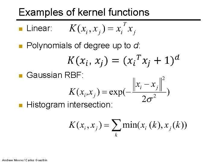
Examples of kernel functions n Linear: n Polynomials of degree up to d: n Gaussian RBF: n Histogram intersection: Andrew Moore / Carlos Guestrin

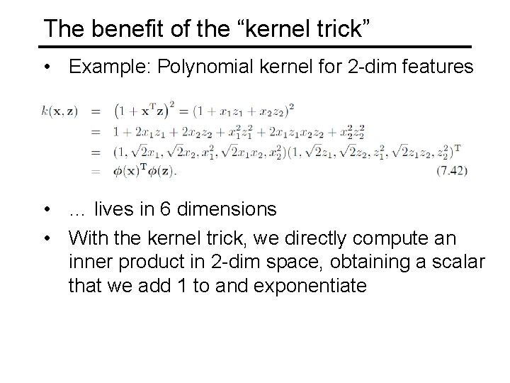
The benefit of the “kernel trick” • Example: Polynomial kernel for 2 -dim features • … lives in 6 dimensions • With the kernel trick, we directly compute an inner product in 2 -dim space, obtaining a scalar that we add 1 to and exponentiate

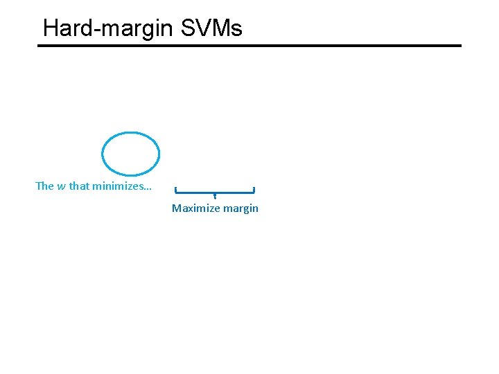
Hard-margin SVMs The w that minimizes… Maximize margin

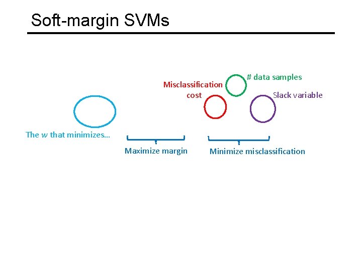
Soft-margin SVMs Misclassification cost # data samples Slack variable The w that minimizes… Maximize margin Minimize misclassification

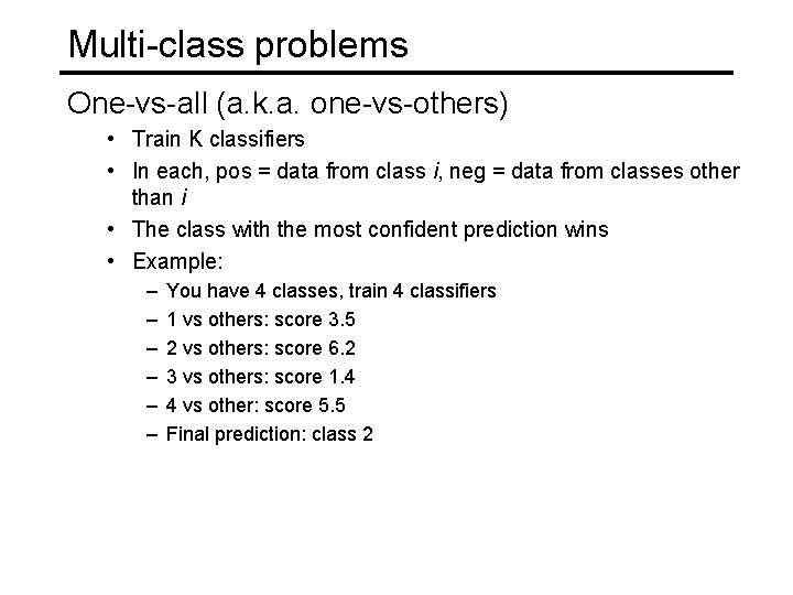
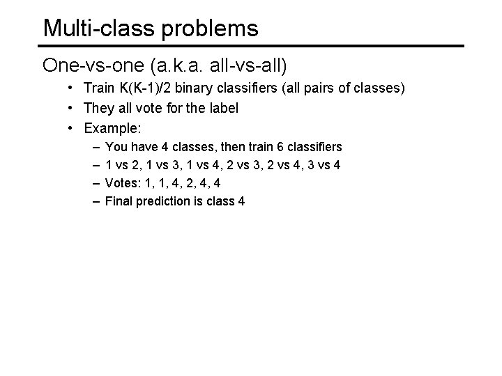
What about multi-class SVMs? • Unfortunately, there is no “definitive” multiclass SVM formulation • In practice, we have to obtain a multi-class SVM by combining multiple two-class SVMs • One vs. others • Training: learn an SVM for each class vs. the others • Testing: apply each SVM to the test example, and assign it to the class of the SVM that returns the highest decision value • One vs. one • Training: learn an SVM for each pair of classes • Testing: each learned SVM “votes” for a class to assign to the test example Svetlana Lazebnik

Multi-class problems One-vs-all (a. k. a. one-vs-others) • Train K classifiers • In each, pos = data from class i, neg = data from classes other than i • The class with the most confident prediction wins • Example: – – – You have 4 classes, train 4 classifiers 1 vs others: score 3. 5 2 vs others: score 6. 2 3 vs others: score 1. 4 4 vs other: score 5. 5 Final prediction: class 2

Multi-class problems One-vs-one (a. k. a. all-vs-all) • Train K(K-1)/2 binary classifiers (all pairs of classes) • They all vote for the label • Example: – – You have 4 classes, then train 6 classifiers 1 vs 2, 1 vs 3, 1 vs 4, 2 vs 3, 2 vs 4, 3 vs 4 Votes: 1, 1, 4, 2, 4, 4 Final prediction is class 4

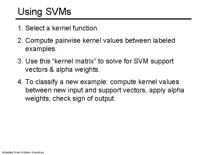
Using SVMs 1. Select a kernel function. 2. Compute pairwise kernel values between labeled examples. 3. Use this “kernel matrix” to solve for SVM support vectors & alpha weights. 4. To classify a new example: compute kernel values between new input and support vectors, apply alpha weights, check sign of output. Adapted from Kristen Grauman

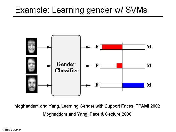
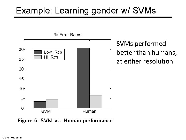
Example: Learning gender w/ SVMs Moghaddam and Yang, Learning Gender with Support Faces, TPAMI 2002 Moghaddam and Yang, Face & Gesture 2000 Kristen Grauman

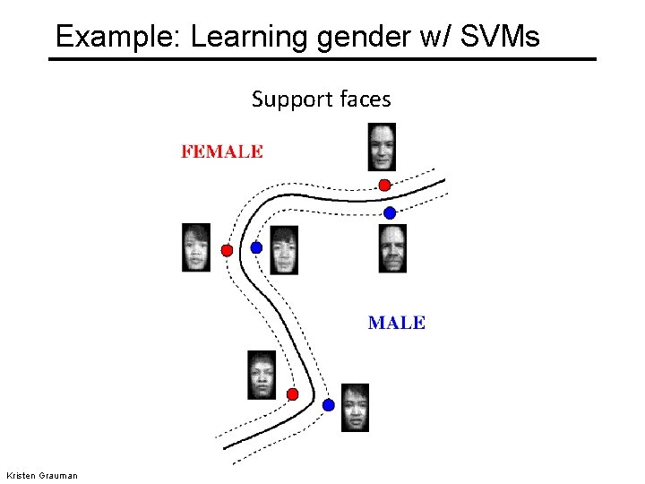
Example: Learning gender w/ SVMs Support faces Kristen Grauman

Example: Learning gender w/ SVMs performed better than humans, at either resolution Kristen Grauman

Some SVM packages • LIBSVM http: //www. csie. ntu. edu. tw/~cjlin/libsvm/ • LIBLINEAR https: //www. csie. ntu. edu. tw/~cjlin/liblinear/ • SVM Light http: //svmlight. joachims. org/

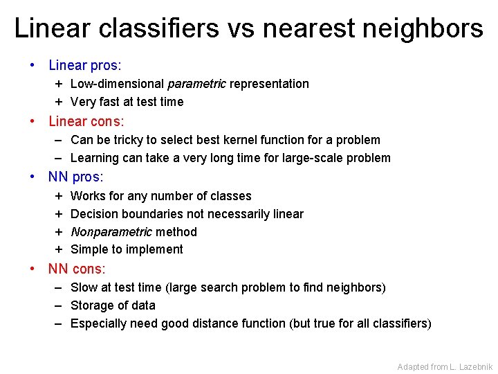
Linear classifiers vs nearest neighbors • Linear pros: + Low-dimensional parametric representation + Very fast at test time • Linear cons: – Can be tricky to select best kernel function for a problem – Learning can take a very long time for large-scale problem • NN pros: + + Works for any number of classes Decision boundaries not necessarily linear Nonparametric method Simple to implement • NN cons: – Slow at test time (large search problem to find neighbors) – Storage of data – Especially need good distance function (but true for all classifiers) Adapted from L. Lazebnik

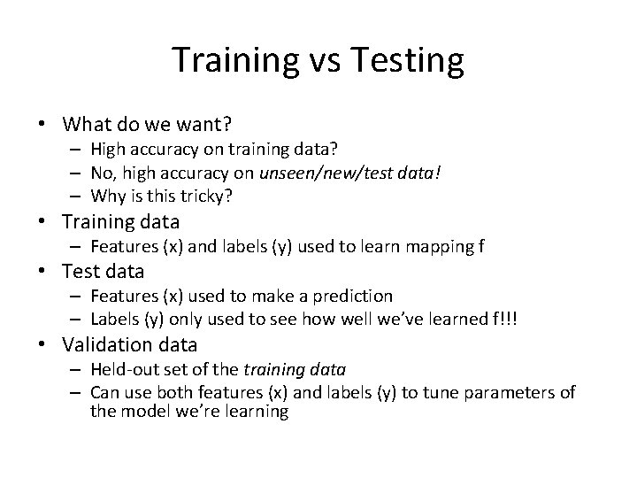
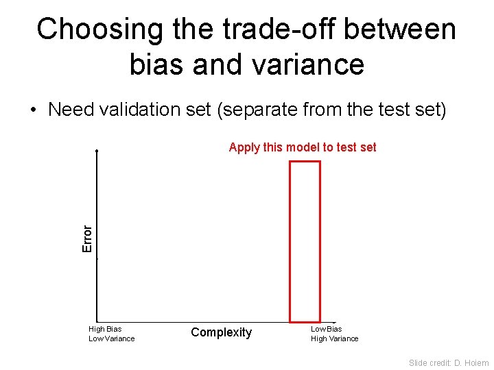
Training vs Testing • What do we want? – High accuracy on training data? – No, high accuracy on unseen/new/test data! – Why is this tricky? • Training data – Features (x) and labels (y) used to learn mapping f • Test data – Features (x) used to make a prediction – Labels (y) only used to see how well we’ve learned f!!! • Validation data – Held-out set of the training data – Can use both features (x) and labels (y) to tune parameters of the model we’re learning

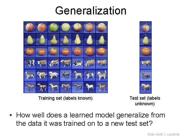
Generalization Training set (labels known) Test set (labels unknown) • How well does a learned model generalize from the data it was trained on to a new test set? Slide credit: L. Lazebnik

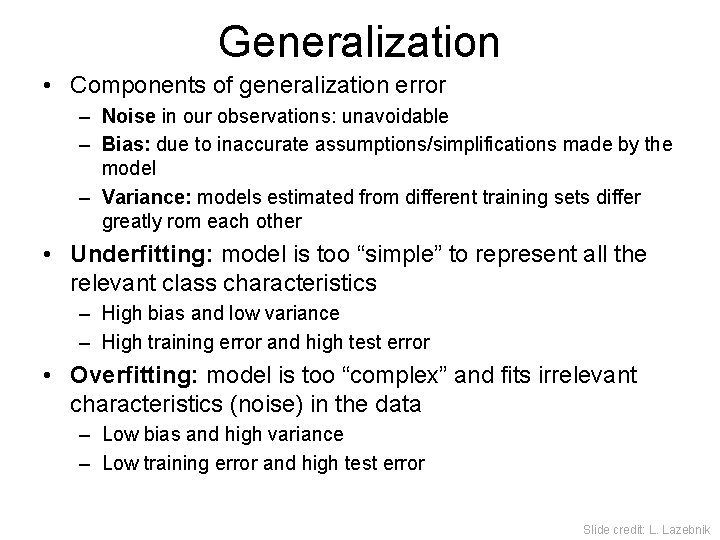
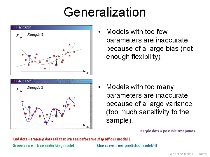
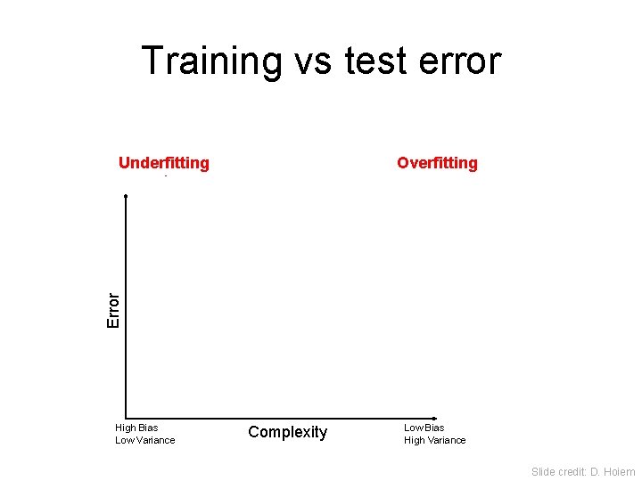
Generalization • Components of generalization error – Noise in our observations: unavoidable – Bias: due to inaccurate assumptions/simplifications made by the model – Variance: models estimated from different training sets differ greatly rom each other • Underfitting: model is too “simple” to represent all the relevant class characteristics – High bias and low variance – High training error and high test error • Overfitting: model is too “complex” and fits irrelevant characteristics (noise) in the data – Low bias and high variance – Low training error and high test error Slide credit: L. Lazebnik

Generalization • Models with too few parameters are inaccurate because of a large bias (not enough flexibility). • Models with too many parameters are inaccurate because of a large variance (too much sensitivity to the sample). Purple dots = possible test points Red dots = training data (all that we see before we ship off our model!) Green curve = true underlying model Blue curve = our predicted model/fit Adapted from D. Hoiem

Training vs test error Overfitting Error Underfitting Test error Training error High Bias Low Variance Complexity Low Bias High Variance Slide credit: D. Hoiem

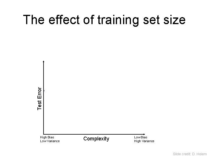
The effect of training set size Test Error Few training examples High Bias Low Variance Many training examples Complexity Low Bias High Variance Slide credit: D. Hoiem

Choosing the trade-off between bias and variance • Need validation set (separate from the test set) Apply this model to test set Error Validation error Training error High Bias Low Variance Complexity Low Bias High Variance Slide credit: D. Hoiem

Generalization tips • Try simple classifiers first • Better to have smart features and simple classifiers than simple features and smart classifiers • Use increasingly powerful classifiers with more training data • As an additional technique for reducing variance, try regularizing the parameters (penalize high magnitude weights) Slide credit: D. Hoiem

Beyond Bags of Features: Spatial Pyramid Matching for Recognizing Natural Scene Categories CVPR 2006 Winner of 2016 Longuet -Higgins Prize Svetlana Lazebnik (slazebni@uiuc. edu) Beckman Institute, University of Illinois at Urbana-Champaign Cordelia Schmid (cordelia. schmid@inrialpes. fr) INRIA Rhône-Alpes, France Jean Ponce (ponce@di. ens. fr) Ecole Normale Supérieure, France

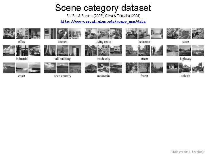
Scene category dataset Fei-Fei & Perona (2005), Oliva & Torralba (2001) http: //www-cvr. ai. uiuc. edu/ponce_grp/data Slide credit: L. Lazebnik

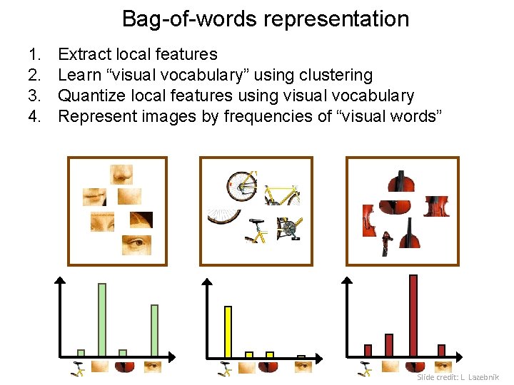
Bag-of-words representation 1. 2. 3. 4. Extract local features Learn “visual vocabulary” using clustering Quantize local features using visual vocabulary Represent images by frequencies of “visual words” Slide credit: L. Lazebnik

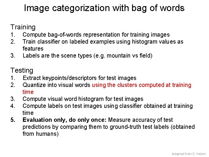
Image categorization with bag of words Training 1. 2. 3. Compute bag-of-words representation for training images Train classifier on labeled examples using histogram values as features Labels are the scene types (e. g. mountain vs field) Testing 1. 2. 3. 4. 5. Extract keypoints/descriptors for test images Quantize into visual words using the clusters computed at training time Compute visual word histogram for test images Compute labels on test images using classifier obtained at training time Evaluation only, do only once: Measure accuracy of test predictions by comparing them to ground-truth test labels (obtained from humans) Adapted from D. Hoiem

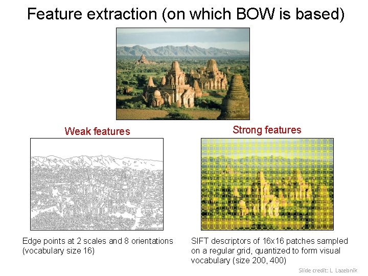
Feature extraction (on which BOW is based) Weak features Edge points at 2 scales and 8 orientations (vocabulary size 16) Strong features SIFT descriptors of 16 x 16 patches sampled on a regular grid, quantized to form visual vocabulary (size 200, 400) Slide credit: L. Lazebnik

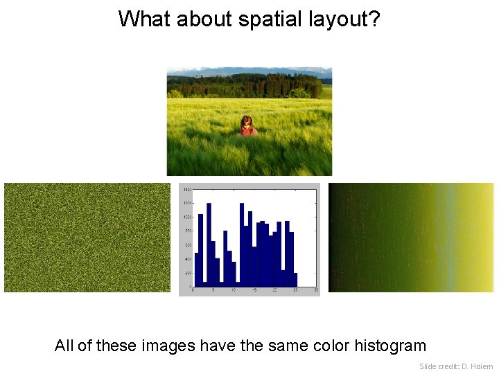
What about spatial layout? All of these images have the same color histogram Slide credit: D. Hoiem

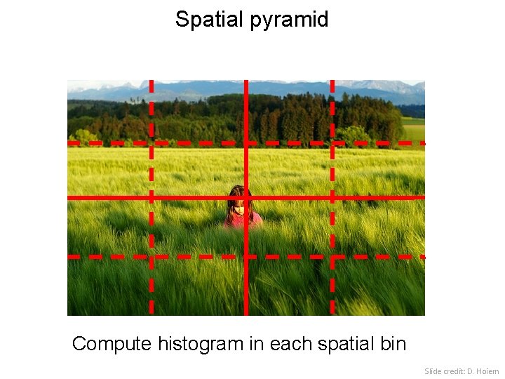
Spatial pyramid Compute histogram in each spatial bin Slide credit: D. Hoiem

Spatial pyramid [Lazebnik et al. CVPR 2006] Slide credit: D. Hoiem

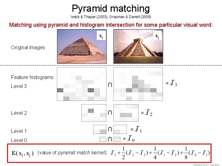
Pyramid matching Indyk & Thaper (2003), Grauman & Darrell (2005) Matching using pyramid and histogram intersection for some particular visual word: xi xj Original images Feature histograms: Level 3 Level 2 Level 1 Level 0 Total weight (value of pyramid match kernel): K( xi , xj ) Adapted from L. Lazebnik

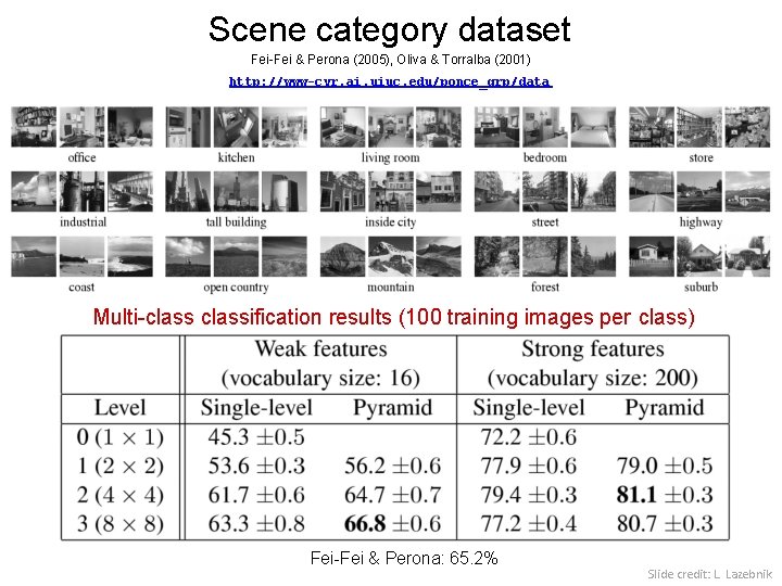
Scene category dataset Fei-Fei & Perona (2005), Oliva & Torralba (2001) http: //www-cvr. ai. uiuc. edu/ponce_grp/data Multi-classification results (100 training images per class) Fei-Fei & Perona: 65. 2% Slide credit: L. Lazebnik

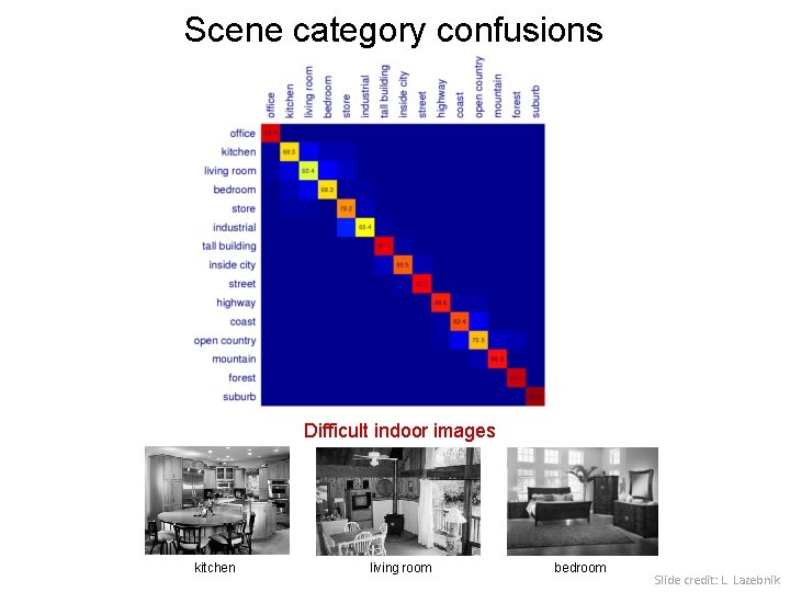
Scene category confusions Difficult indoor images kitchen living room bedroom Slide credit: L. Lazebnik

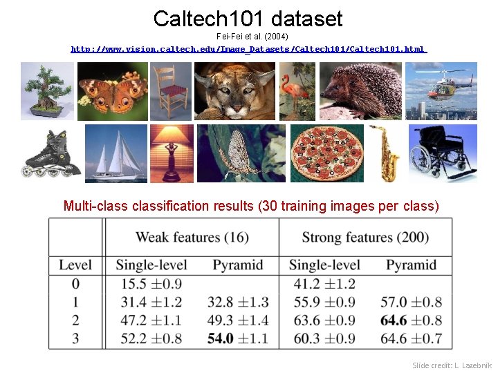
Caltech 101 dataset Fei-Fei et al. (2004) http: //www. vision. caltech. edu/Image_Datasets/Caltech 101. html Multi-classification results (30 training images per class) Slide credit: L. Lazebnik