CS 2770 Computer Vision Intro to Visual Recognition

CS 2770: Computer Vision Intro to Visual Recognition Prof. Adriana Kovashka University of Pittsburgh February 13, 2018

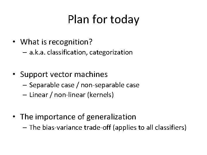
Plan for today • What is recognition? – a. k. a. classification, categorization • Support vector machines – Separable case / non-separable case – Linear / non-linear (kernels) • The importance of generalization – The bias-variance trade-off (applies to all classifiers)

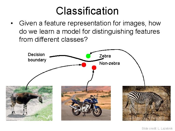
Classification • Given a feature representation for images, how do we learn a model for distinguishing features from different classes? Decision boundary Zebra Non-zebra Slide credit: L. Lazebnik

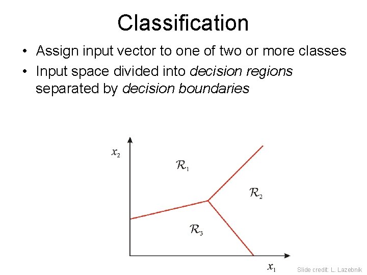
Classification • Assign input vector to one of two or more classes • Input space divided into decision regions separated by decision boundaries Slide credit: L. Lazebnik

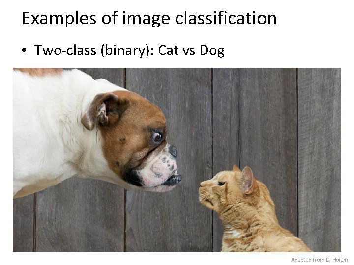
Examples of image classification • Two-class (binary): Cat vs Dog Adapted from D. Hoiem

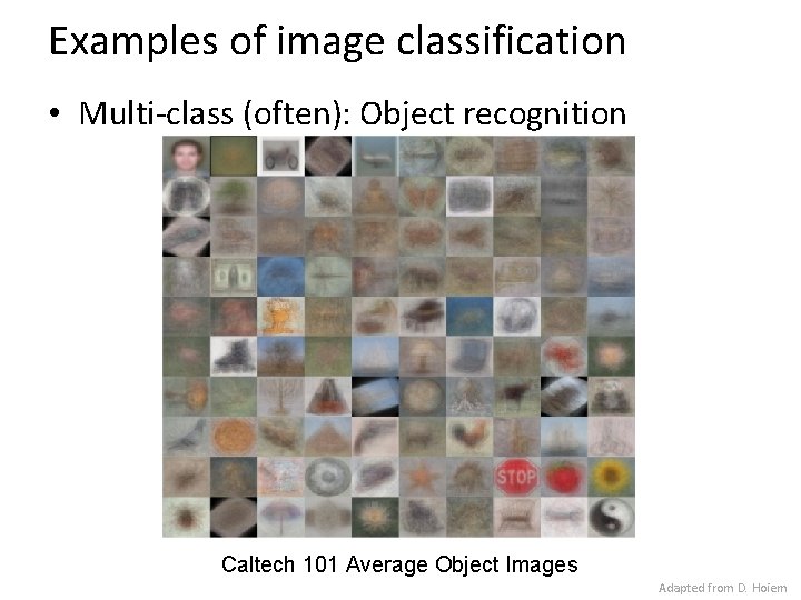
Examples of image classification • Multi-class (often): Object recognition Caltech 101 Average Object Images Adapted from D. Hoiem

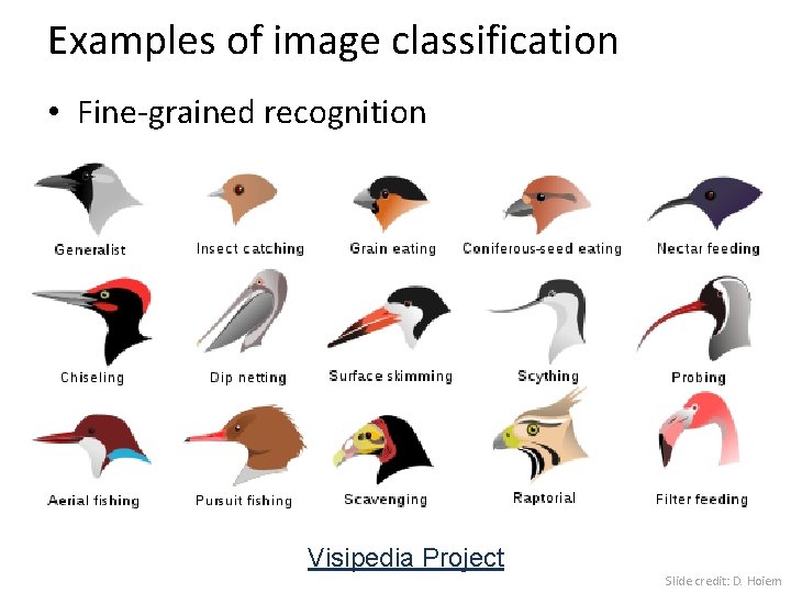
Examples of image classification • Fine-grained recognition Visipedia Project Slide credit: D. Hoiem

Examples of image classification • Place recognition Places Database [Zhou et al. NIPS 2014] Slide credit: D. Hoiem

Examples of image classification • Material recognition [Bell et al. CVPR 2015] Slide credit: D. Hoiem

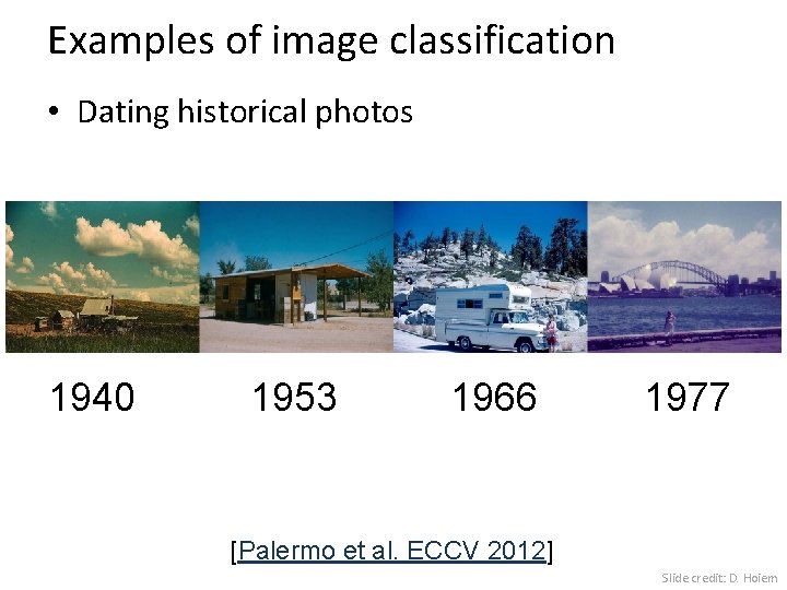
Examples of image classification • Dating historical photos 1940 1953 1966 1977 [Palermo et al. ECCV 2012] Slide credit: D. Hoiem

Examples of image classification • Image style recognition [Karayev et al. BMVC 2014] Slide credit: D. Hoiem

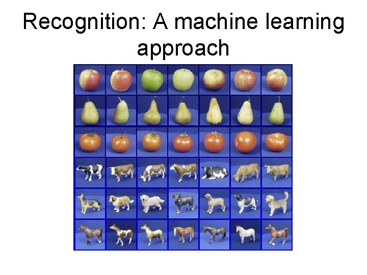
Recognition: A machine learning approach

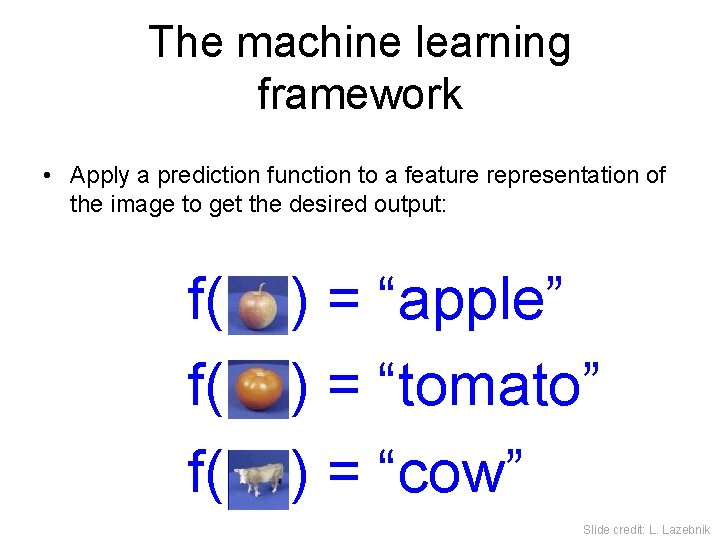
The machine learning framework • Apply a prediction function to a feature representation of the image to get the desired output: f( ) = “apple” f( ) = “tomato” f( ) = “cow” Slide credit: L. Lazebnik

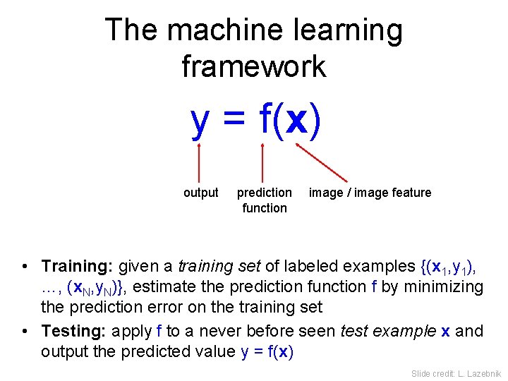
The machine learning framework y = f(x) output prediction function image / image feature • Training: given a training set of labeled examples {(x 1, y 1), …, (x. N, y. N)}, estimate the prediction function f by minimizing the prediction error on the training set • Testing: apply f to a never before seen test example x and output the predicted value y = f(x) Slide credit: L. Lazebnik

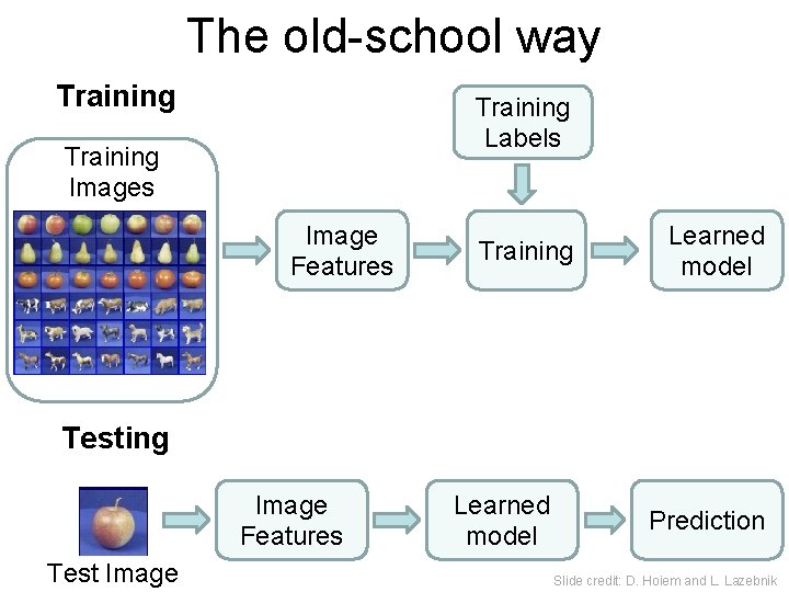
The old-school way Training Labels Training Images Image Features Training Learned model Testing Image Features Test Image Learned model Prediction Slide credit: D. Hoiem and L. Lazebnik

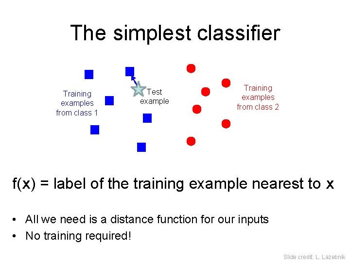
The simplest classifier Training examples from class 1 Test example Training examples from class 2 f(x) = label of the training example nearest to x • All we need is a distance function for our inputs • No training required! Slide credit: L. Lazebnik

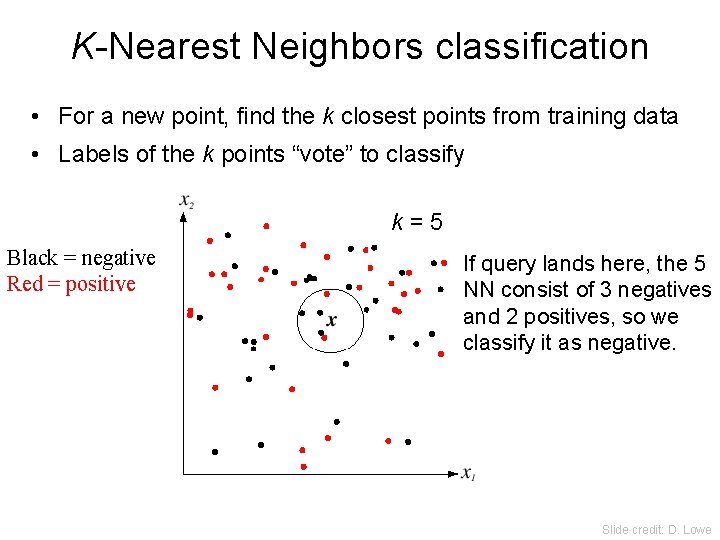
K-Nearest Neighbors classification • For a new point, find the k closest points from training data • Labels of the k points “vote” to classify k = 5 Black = negative Red = positive If query lands here, the 5 NN consist of 3 negatives and 2 positives, so we classify it as negative. Slide credit: D. Lowe

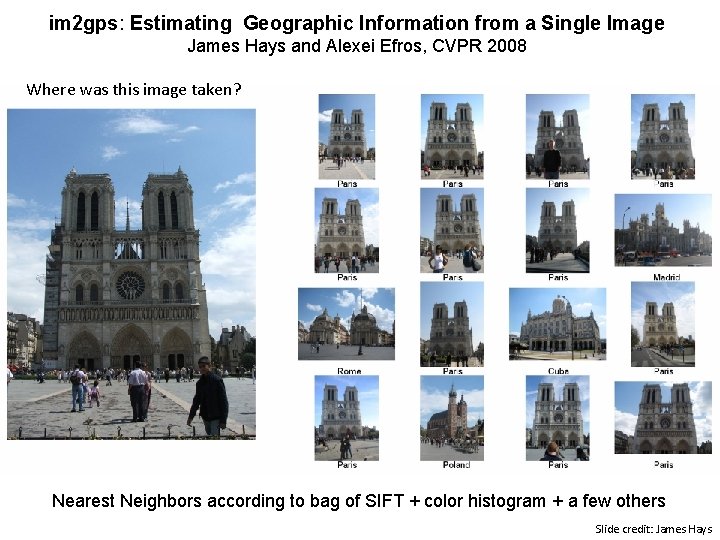
im 2 gps: Estimating Geographic Information from a Single Image James Hays and Alexei Efros, CVPR 2008 Where was this image taken? Nearest Neighbors according to bag of SIFT + color histogram + a few others Slide credit: James Hays

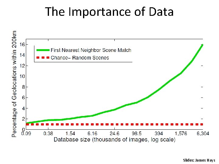
The Importance of Data Slides: James Hays

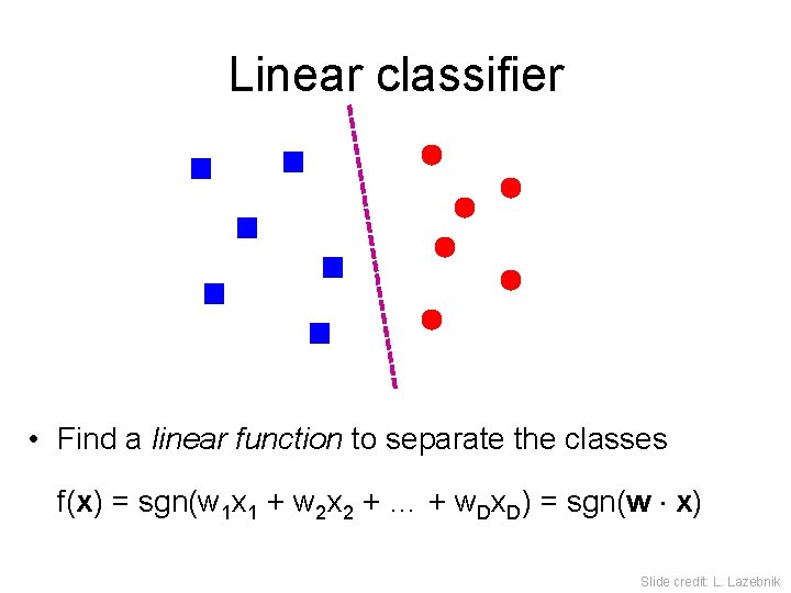
Linear classifier • Find a linear function to separate the classes f(x) = sgn(w 1 x 1 + w 2 x 2 + … + w. Dx. D) = sgn(w x) Slide credit: L. Lazebnik

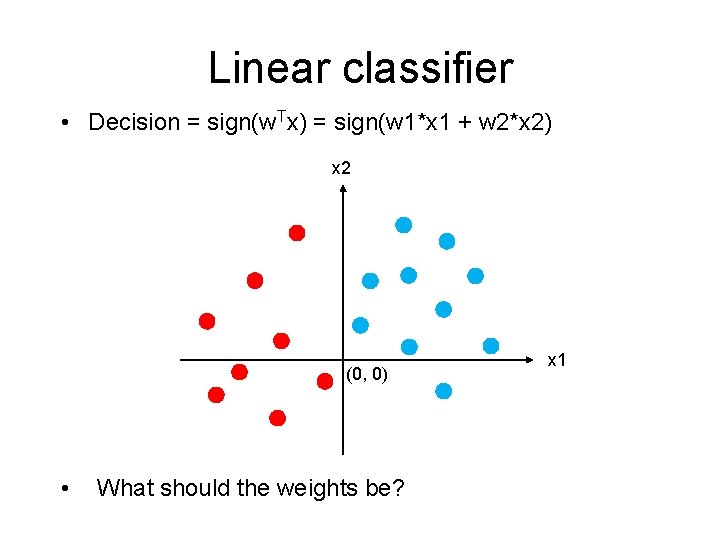
Linear classifier • Decision = sign(w. Tx) = sign(w 1*x 1 + w 2*x 2) x 2 (0, 0) • What should the weights be? x 1

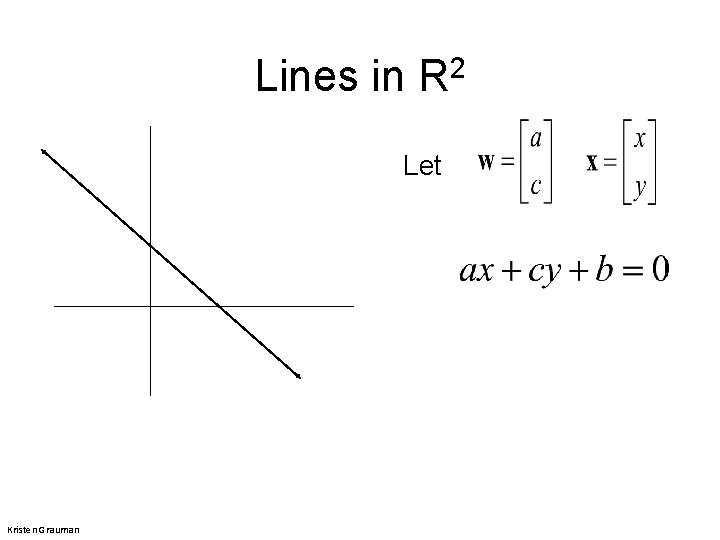
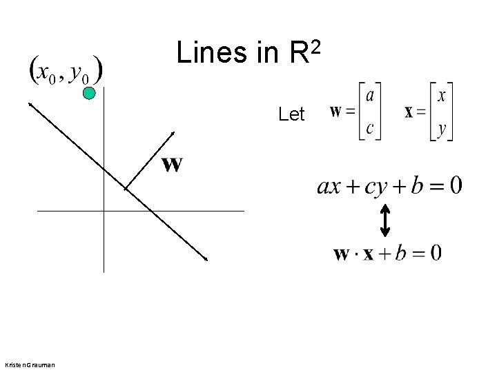
Lines in R 2 Let Kristen Grauman

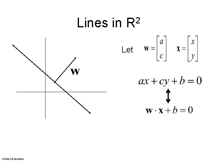
Lines in R 2 Let Kristen Grauman

Lines in R 2 Let Kristen Grauman

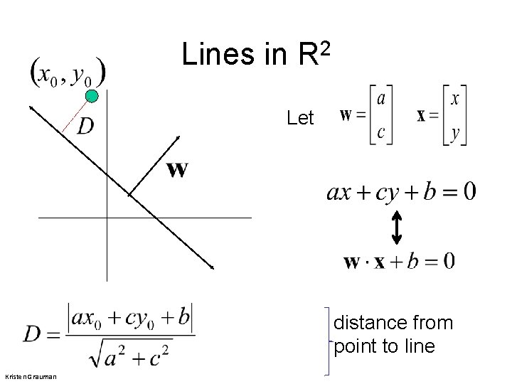
Lines in R 2 Let distance from point to line Kristen Grauman

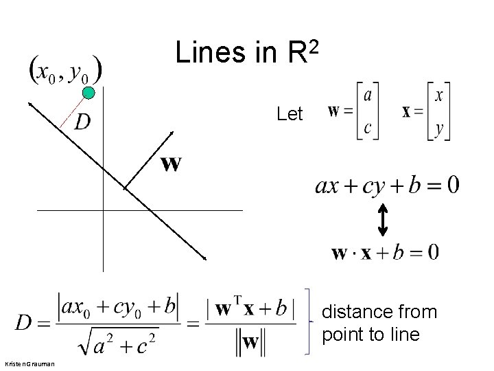
Lines in R 2 Let distance from point to line Kristen Grauman

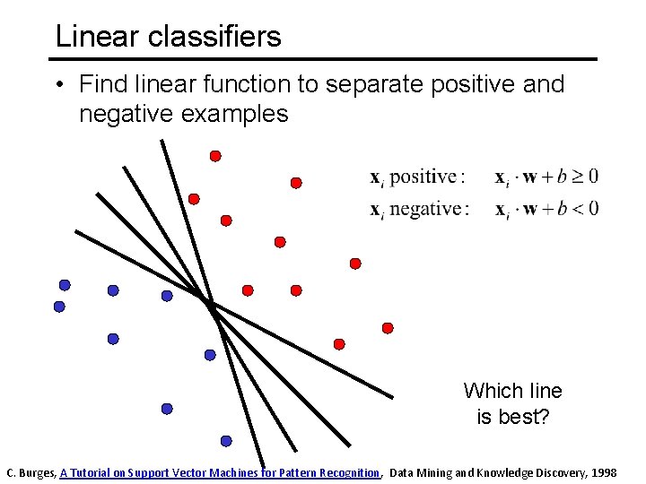
Linear classifiers • Find linear function to separate positive and negative examples Which line is best? C. Burges, A Tutorial on Support Vector Machines for Pattern Recognition, Data Mining and Knowledge Discovery, 1998

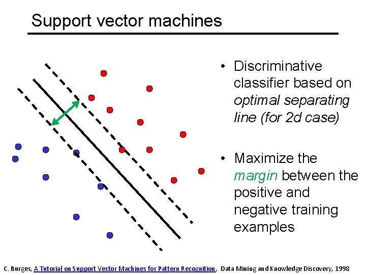
Support vector machines • Discriminative classifier based on optimal separating line (for 2 d case) • Maximize the margin between the positive and negative training examples C. Burges, A Tutorial on Support Vector Machines for Pattern Recognition, Data Mining and Knowledge Discovery, 1998

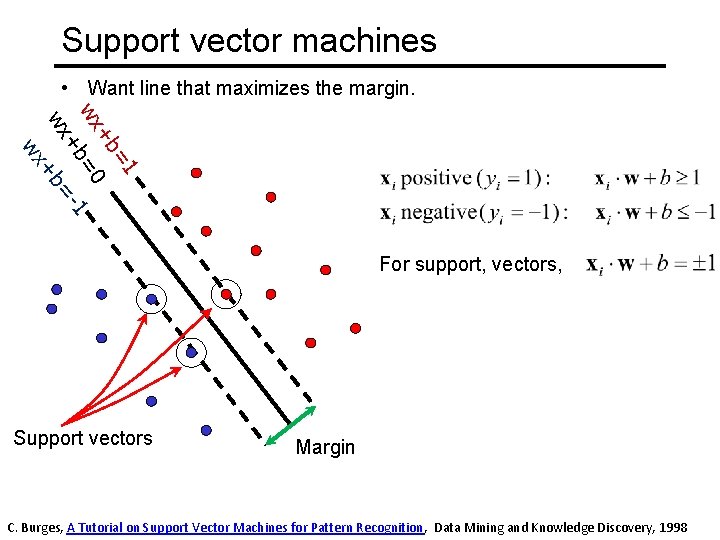
Support vector machines • Want line that maximizes the margin. =1 +b wx =0 1 +b wx +b= wx For support, vectors, Support vectors Margin C. Burges, A Tutorial on Support Vector Machines for Pattern Recognition, Data Mining and Knowledge Discovery, 1998

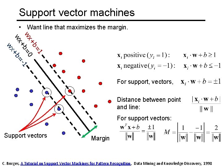
Support vector machines • Want line that maximizes the margin. =1 +b wx =0 1 +b wx +b= wx For support, vectors, Distance between point and line: For support vectors: Support vectors Margin C. Burges, A Tutorial on Support Vector Machines for Pattern Recognition, Data Mining and Knowledge Discovery, 1998

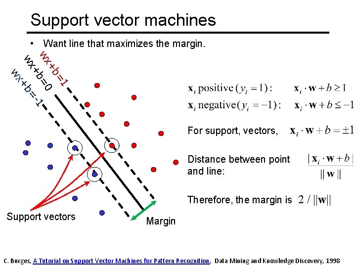
Support vector machines • Want line that maximizes the margin. =1 +b wx =0 1 +b wx +b= wx For support, vectors, Distance between point and line: Therefore, the margin is 2 Support vectors / ||w|| Margin C. Burges, A Tutorial on Support Vector Machines for Pattern Recognition, Data Mining and Knowledge Discovery, 1998

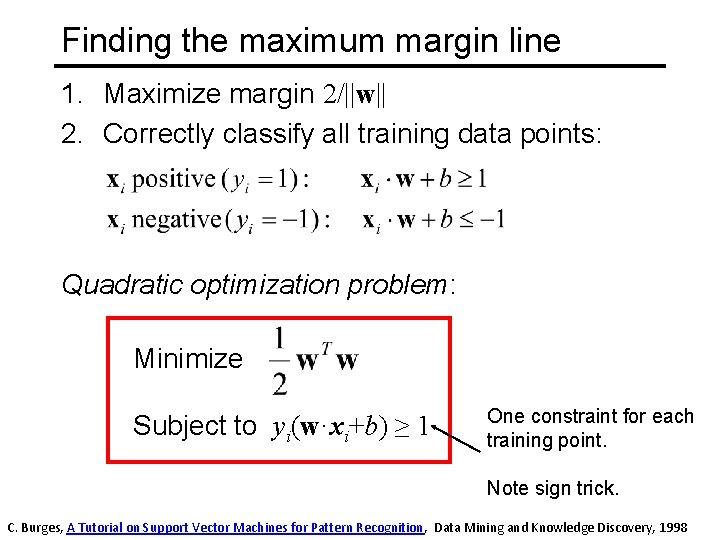
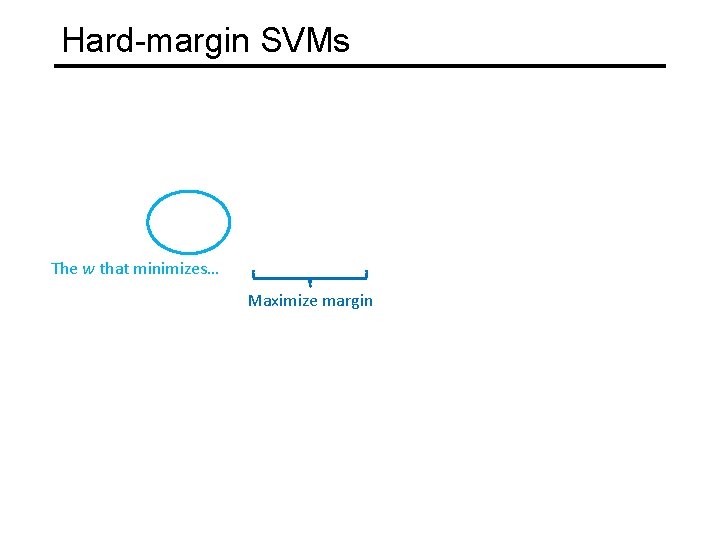
Finding the maximum margin line 1. Maximize margin 2/||w|| 2. Correctly classify all training data points: Quadratic optimization problem: Minimize Subject to yi(w·xi+b) ≥ 1 One constraint for each training point. Note sign trick. C. Burges, A Tutorial on Support Vector Machines for Pattern Recognition, Data Mining and Knowledge Discovery, 1998

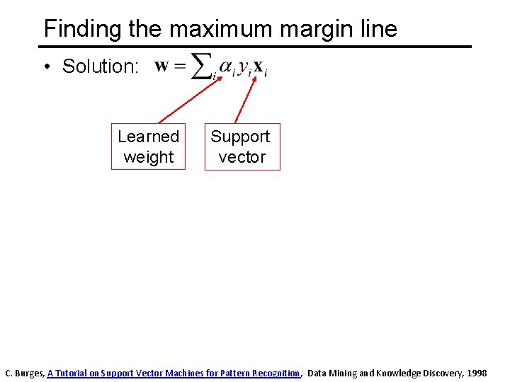
Finding the maximum margin line • Solution: Learned weight Support vector C. Burges, A Tutorial on Support Vector Machines for Pattern Recognition, Data Mining and Knowledge Discovery, 1998

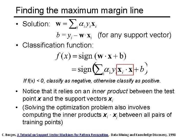
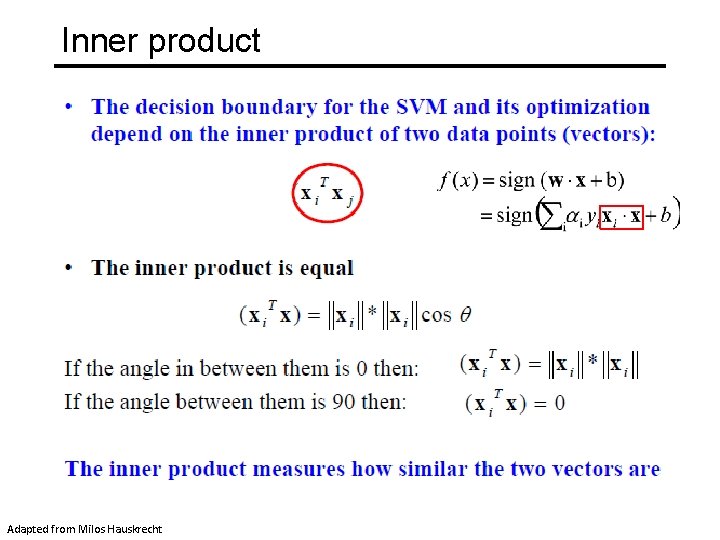
Finding the maximum margin line • Solution: b = yi – w·xi (for any support vector) • Classification function: If f(x) < 0, classify as negative, otherwise classify as positive. • Notice that it relies on an inner product between the test point x and the support vectors xi • (Solving the optimization problem also involves computing the inner products xi · xj between all pairs of training points) C. Burges, A Tutorial on Support Vector Machines for Pattern Recognition, Data Mining and Knowledge Discovery, 1998

Inner product Adapted from Milos Hauskrecht

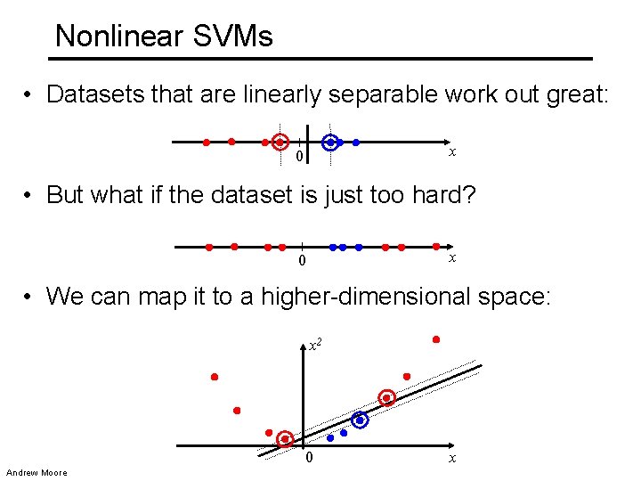
Nonlinear SVMs • Datasets that are linearly separable work out great: x 0 • But what if the dataset is just too hard? x 0 • We can map it to a higher-dimensional space: x 2 0 Andrew Moore x

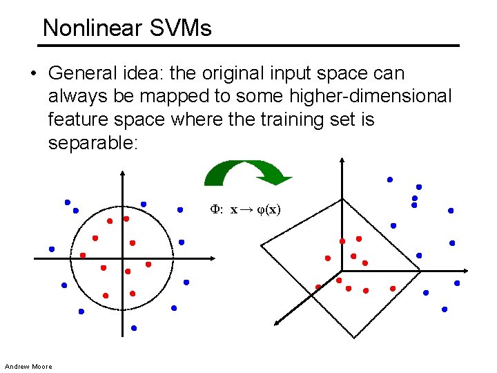
Nonlinear SVMs • General idea: the original input space can always be mapped to some higher-dimensional feature space where the training set is separable: Φ: x → φ(x) Andrew Moore

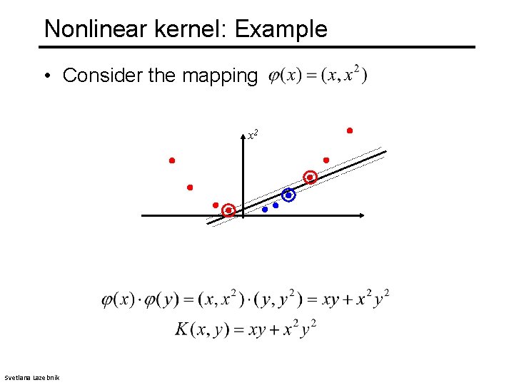
Nonlinear kernel: Example • Consider the mapping x 2 Svetlana Lazebnik

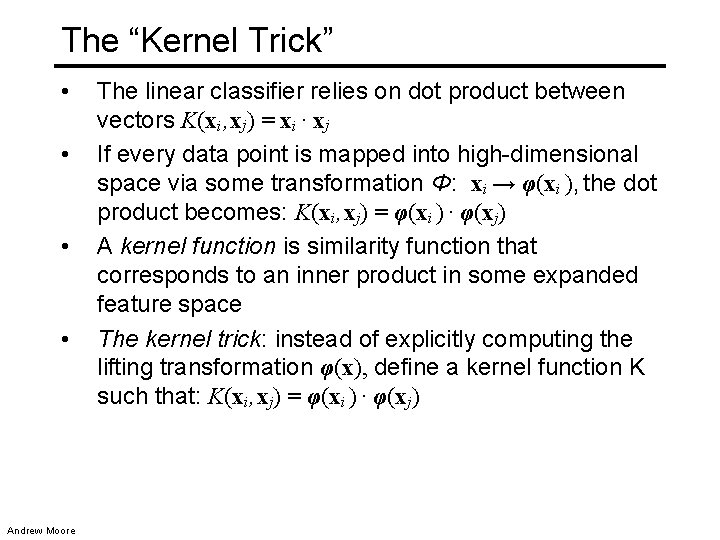
The “Kernel Trick” • • Andrew Moore The linear classifier relies on dot product between vectors K(xi , xj) = xi · xj If every data point is mapped into high-dimensional space via some transformation Φ: xi → φ(xi ), the dot product becomes: K(xi , xj) = φ(xi ) · φ(xj) A kernel function is similarity function that corresponds to an inner product in some expanded feature space The kernel trick: instead of explicitly computing the lifting transformation φ(x), define a kernel function K such that: K(xi , xj) = φ(xi ) · φ(xj)

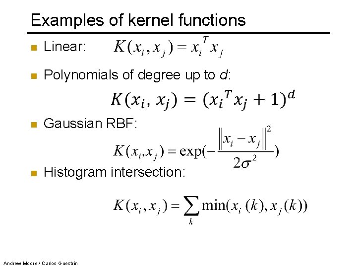
Examples of kernel functions n Linear: n Polynomials of degree up to d: n Gaussian RBF: n Histogram intersection: Andrew Moore / Carlos Guestrin

Hard-margin SVMs The w that minimizes… Maximize margin

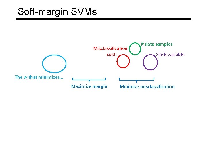
Soft-margin SVMs Misclassification cost # data samples Slack variable The w that minimizes… Maximize margin Minimize misclassification

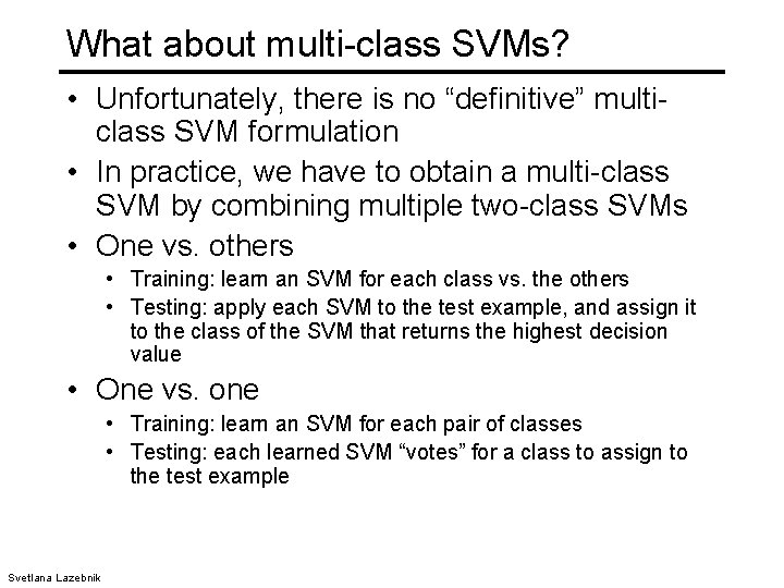
What about multi-class SVMs? • Unfortunately, there is no “definitive” multiclass SVM formulation • In practice, we have to obtain a multi-class SVM by combining multiple two-class SVMs • One vs. others • Training: learn an SVM for each class vs. the others • Testing: apply each SVM to the test example, and assign it to the class of the SVM that returns the highest decision value • One vs. one • Training: learn an SVM for each pair of classes • Testing: each learned SVM “votes” for a class to assign to the test example Svetlana Lazebnik

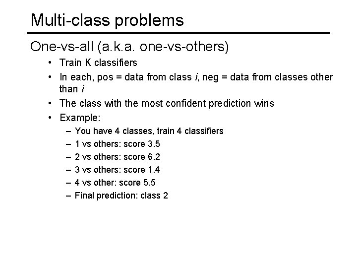
Multi-class problems One-vs-all (a. k. a. one-vs-others) • Train K classifiers • In each, pos = data from class i, neg = data from classes other than i • The class with the most confident prediction wins • Example: – – – You have 4 classes, train 4 classifiers 1 vs others: score 3. 5 2 vs others: score 6. 2 3 vs others: score 1. 4 4 vs other: score 5. 5 Final prediction: class 2

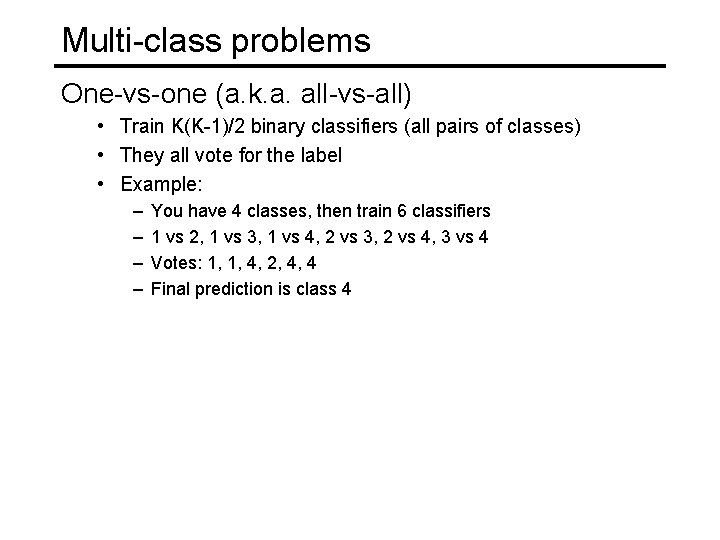
Multi-class problems One-vs-one (a. k. a. all-vs-all) • Train K(K-1)/2 binary classifiers (all pairs of classes) • They all vote for the label • Example: – – You have 4 classes, then train 6 classifiers 1 vs 2, 1 vs 3, 1 vs 4, 2 vs 3, 2 vs 4, 3 vs 4 Votes: 1, 1, 4, 2, 4, 4 Final prediction is class 4

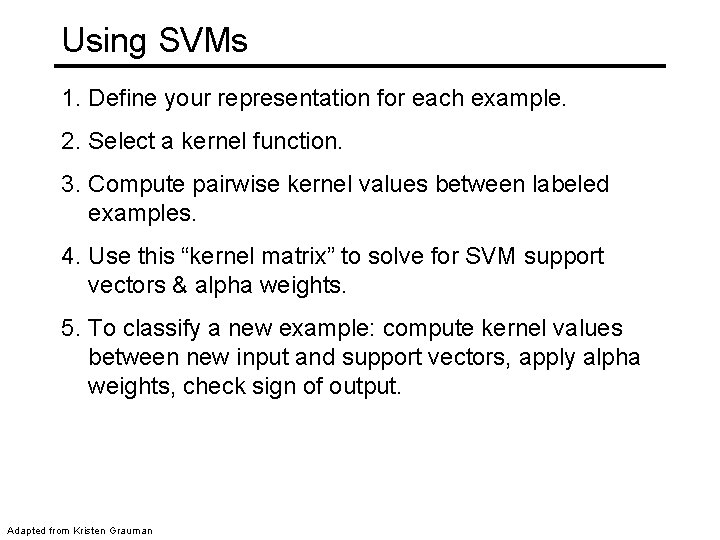
Using SVMs 1. Define your representation for each example. 2. Select a kernel function. 3. Compute pairwise kernel values between labeled examples. 4. Use this “kernel matrix” to solve for SVM support vectors & alpha weights. 5. To classify a new example: compute kernel values between new input and support vectors, apply alpha weights, check sign of output. Adapted from Kristen Grauman

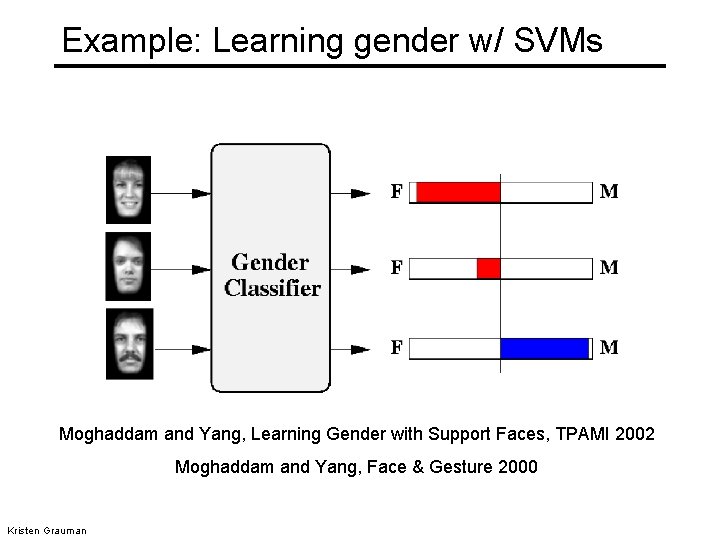
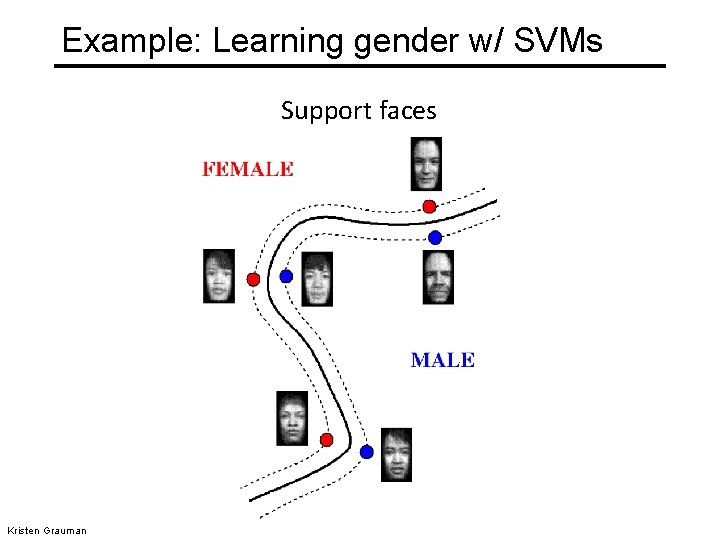
Example: Learning gender w/ SVMs Moghaddam and Yang, Learning Gender with Support Faces, TPAMI 2002 Moghaddam and Yang, Face & Gesture 2000 Kristen Grauman

Example: Learning gender w/ SVMs Support faces Kristen Grauman

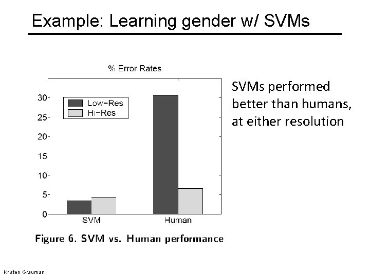
Example: Learning gender w/ SVMs performed better than humans, at either resolution Kristen Grauman

Some SVM packages • LIBSVM http: //www. csie. ntu. edu. tw/~cjlin/libsvm/ • LIBLINEAR https: //www. csie. ntu. edu. tw/~cjlin/liblinear/ • SVM Light http: //svmlight. joachims. org/

Linear classifiers vs nearest neighbors • Linear pros: + Low-dimensional parametric representation + Very fast at test time • Linear cons: – Can be tricky to select best kernel function for a problem – Learning can take a very long time for large-scale problem • NN pros: + + Works for any number of classes Decision boundaries not necessarily linear Nonparametric method Simple to implement • NN cons: – Slow at test time (large search problem to find neighbors) – Storage of data – Especially need good distance function (but true for all classifiers) Adapted from L. Lazebnik

Training vs Testing • What do we want? – High accuracy on training data? – No, high accuracy on unseen/new/test data! – Why is this tricky? • Training data – Features (x) and labels (y) used to learn mapping f • Test data – Features (x) used to make a prediction – Labels (y) only used to see how well we’ve learned f!!! • Validation data – Held-out set of the training data – Can use both features (x) and labels (y) to tune parameters of the model we’re learning

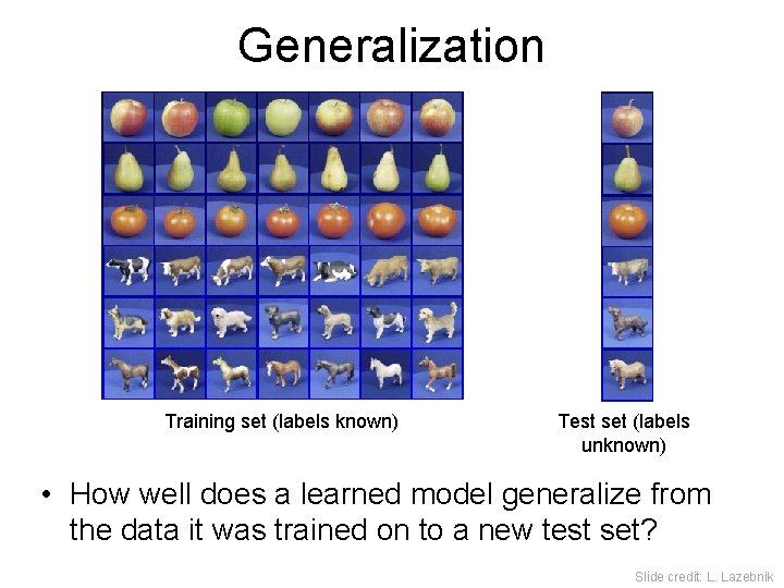
Generalization Training set (labels known) Test set (labels unknown) • How well does a learned model generalize from the data it was trained on to a new test set? Slide credit: L. Lazebnik

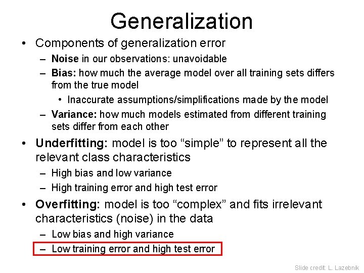
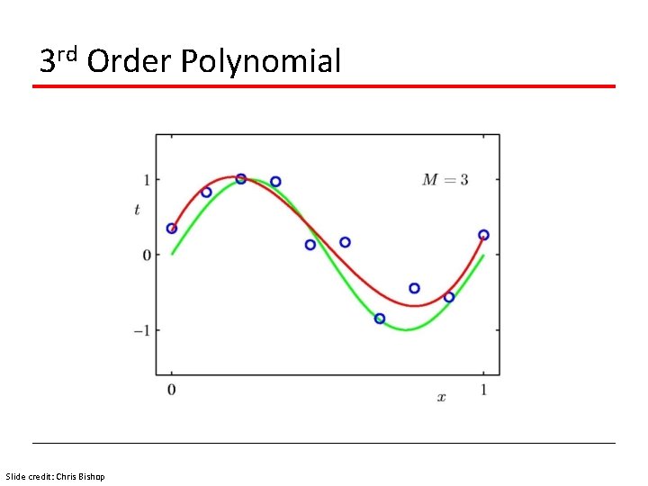
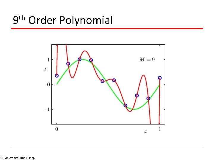
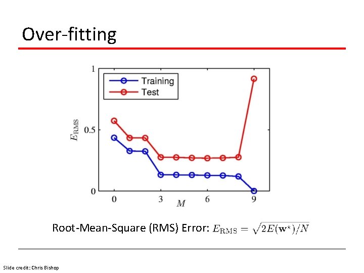
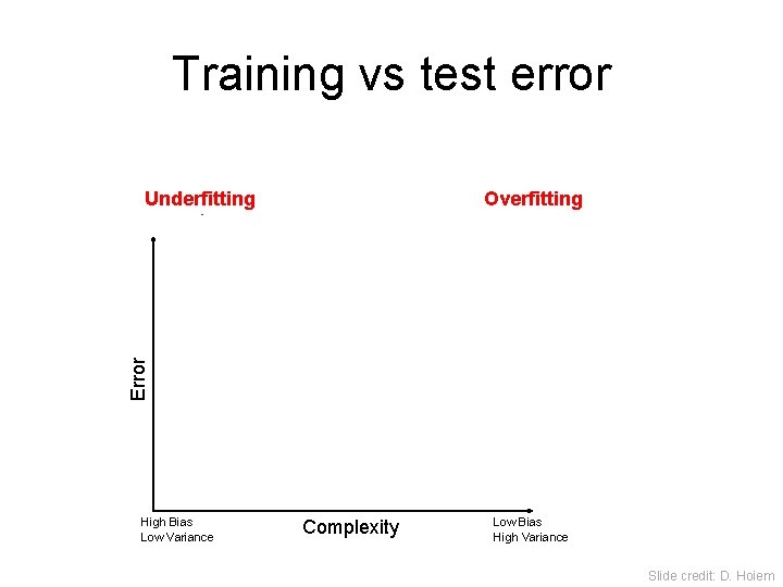
Generalization • Components of generalization error – Noise in our observations: unavoidable – Bias: how much the average model over all training sets differs from the true model • Inaccurate assumptions/simplifications made by the model – Variance: how much models estimated from different training sets differ from each other • Underfitting: model is too “simple” to represent all the relevant class characteristics – High bias and low variance – High training error and high test error • Overfitting: model is too “complex” and fits irrelevant characteristics (noise) in the data – Low bias and high variance – Low training error and high test error Slide credit: L. Lazebnik

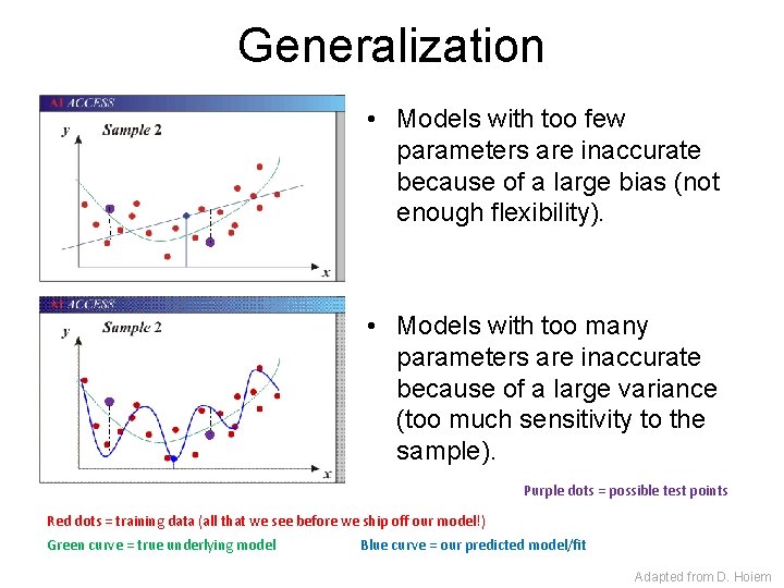
Generalization • Models with too few parameters are inaccurate because of a large bias (not enough flexibility). • Models with too many parameters are inaccurate because of a large variance (too much sensitivity to the sample). Purple dots = possible test points Red dots = training data (all that we see before we ship off our model!) Green curve = true underlying model Blue curve = our predicted model/fit Adapted from D. Hoiem

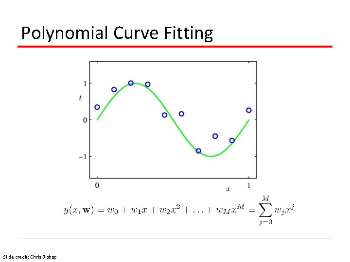
Polynomial Curve Fitting Slide credit: Chris Bishop

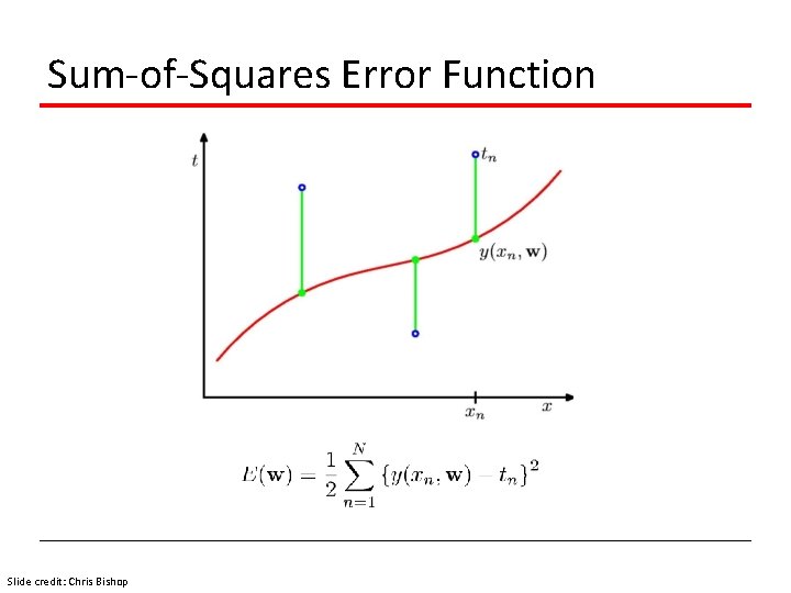
Sum-of-Squares Error Function Slide credit: Chris Bishop

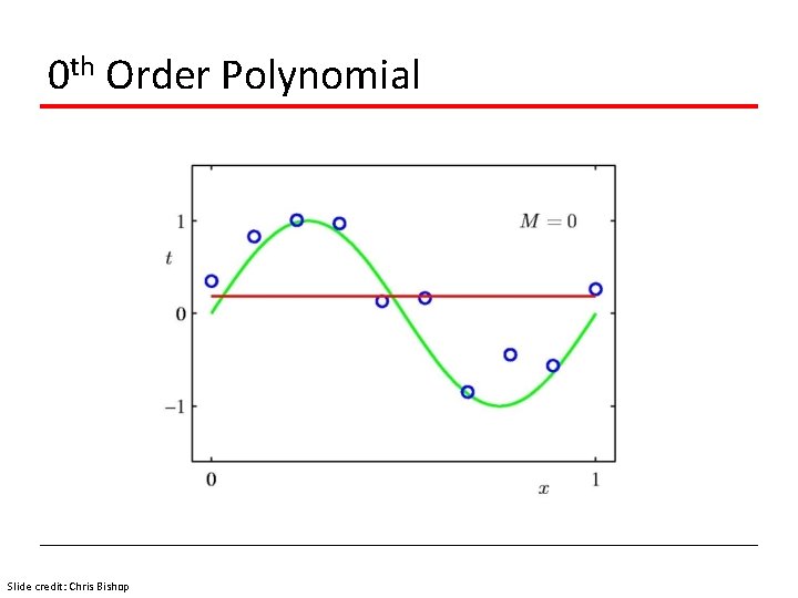
0 th Order Polynomial Slide credit: Chris Bishop

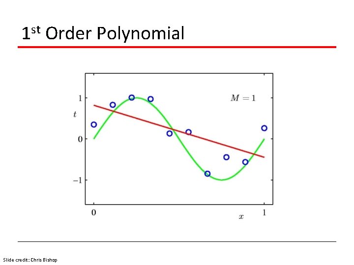
1 st Order Polynomial Slide credit: Chris Bishop

3 rd Order Polynomial Slide credit: Chris Bishop

9 th Order Polynomial Slide credit: Chris Bishop

Over-fitting Root-Mean-Square (RMS) Error: Slide credit: Chris Bishop

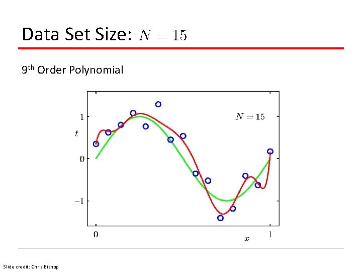
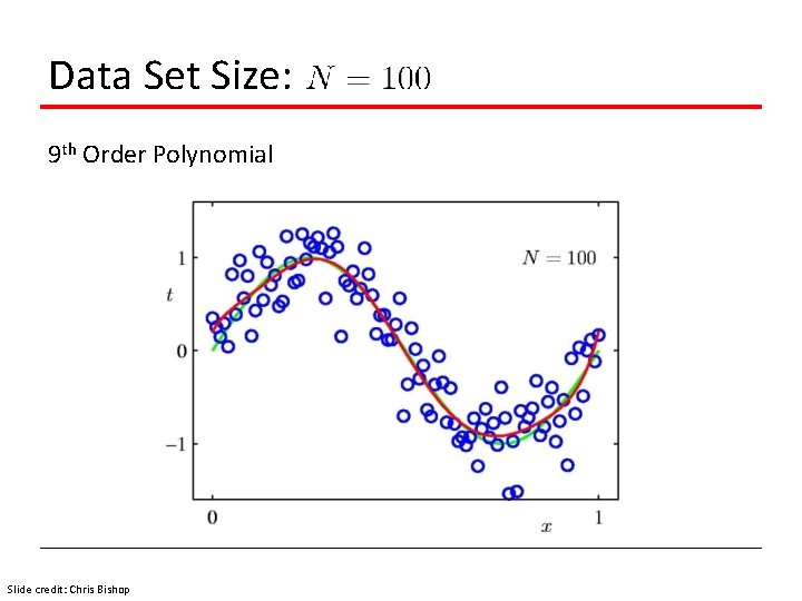
Data Set Size: 9 th Order Polynomial Slide credit: Chris Bishop

Data Set Size: 9 th Order Polynomial Slide credit: Chris Bishop

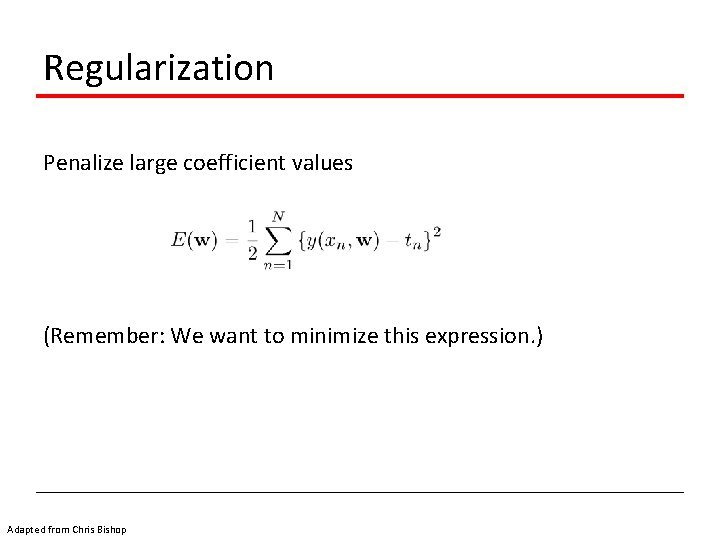
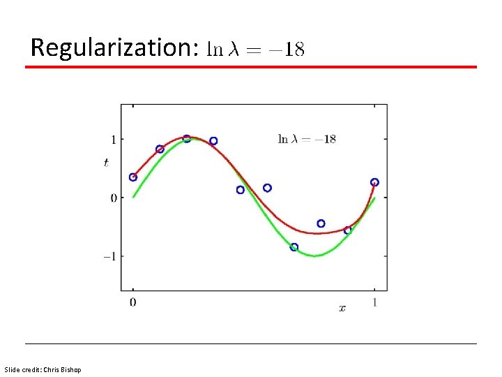
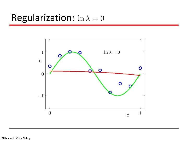
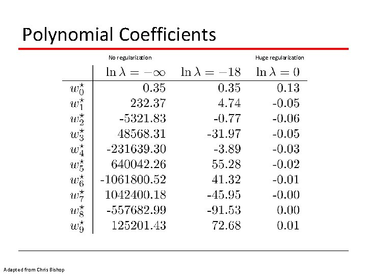
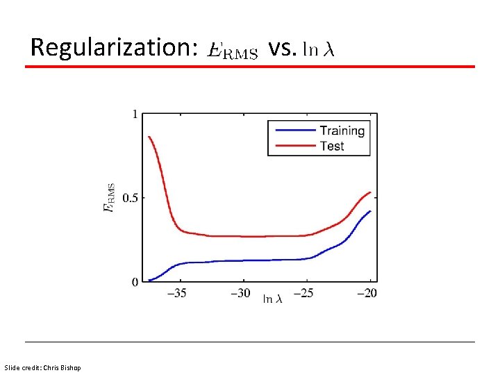
Regularization Penalize large coefficient values (Remember: We want to minimize this expression. ) Adapted from Chris Bishop

Regularization: Slide credit: Chris Bishop

Regularization: Slide credit: Chris Bishop

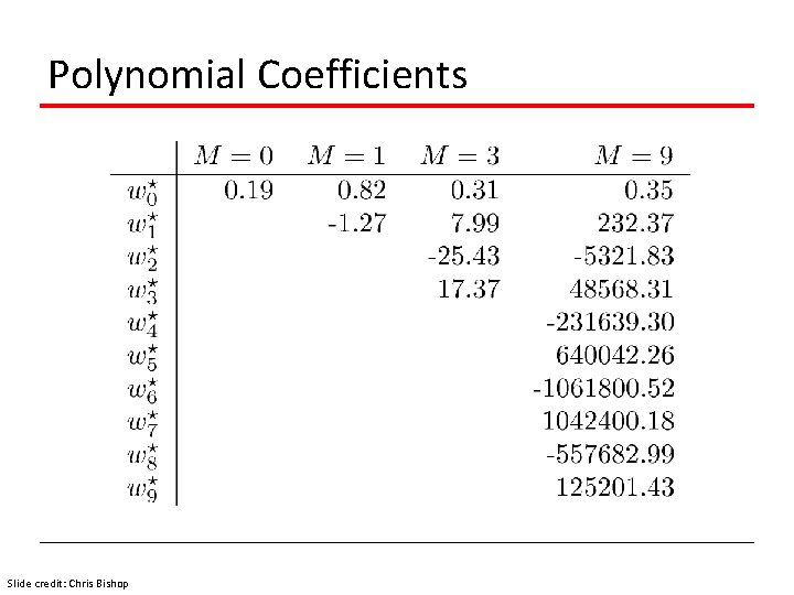
Polynomial Coefficients Slide credit: Chris Bishop

Polynomial Coefficients No regularization Adapted from Chris Bishop Huge regularization

Regularization: Slide credit: Chris Bishop vs.

Training vs test error Overfitting Error Underfitting Test error Training error High Bias Low Variance Complexity Low Bias High Variance Slide credit: D. Hoiem

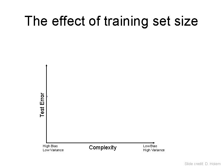
The effect of training set size Test Error Few training examples High Bias Low Variance Many training examples Complexity Low Bias High Variance Slide credit: D. Hoiem

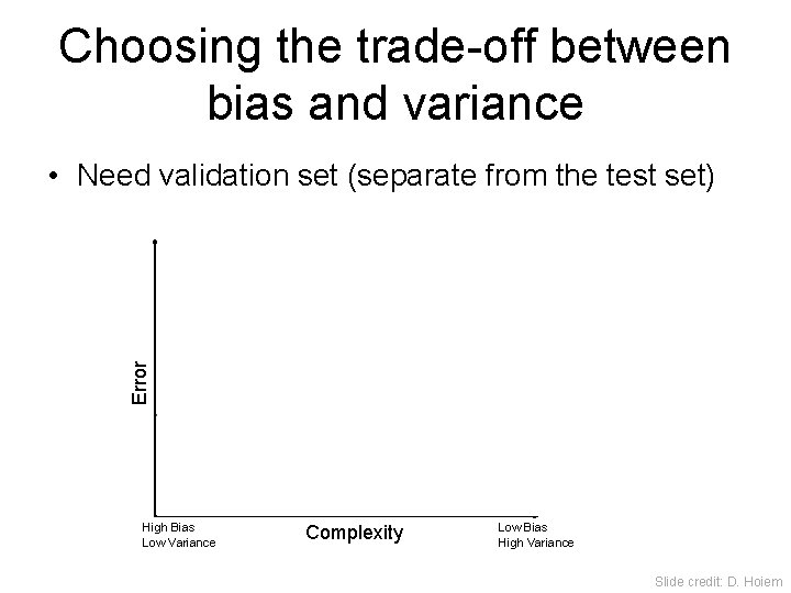
Choosing the trade-off between bias and variance • Need validation set (separate from the test set) Error Validation error Training error High Bias Low Variance Complexity Low Bias High Variance Slide credit: D. Hoiem

Summary • Try simple classifiers first • Better to have smart features and simple classifiers than simple features and smart classifiers • Use increasingly powerful classifiers with more training data • As an additional technique for reducing variance, try regularizing the parameters Slide credit: D. Hoiem