CS 1674 Intro to Computer Vision Local Feature

CS 1674: Intro to Computer Vision Local Feature Detection Prof. Adriana Kovashka University of Pittsburgh September 19, 2016

Announcements • HW 1 P, HW 2 W graded

Notes on HW 2 W • Graded with some comments on submission itself Please read my feedback • I didn’t respond to you on the last 2 questions, my silence does not mean you’re correct • Try to be concise, without failing to give me the answer • If you have 12 or less, you should be concerned • The book is often a useful resource • Laplacian vs Sobel (hw 2 w. m)

Note on assignments • Lots of questions about “is it ok if I do this” – You don’t have to worry so much about doing exactly what I said, as long as you do the core task of the assignment! – After HW 1 P, it doesn’t matter how you print, or whether you put multiple figures in one, etc.

HW 2 P post-mortem • • How long did it take? What took the most time? What was most fun? What was most annoying? • Enter Socrative

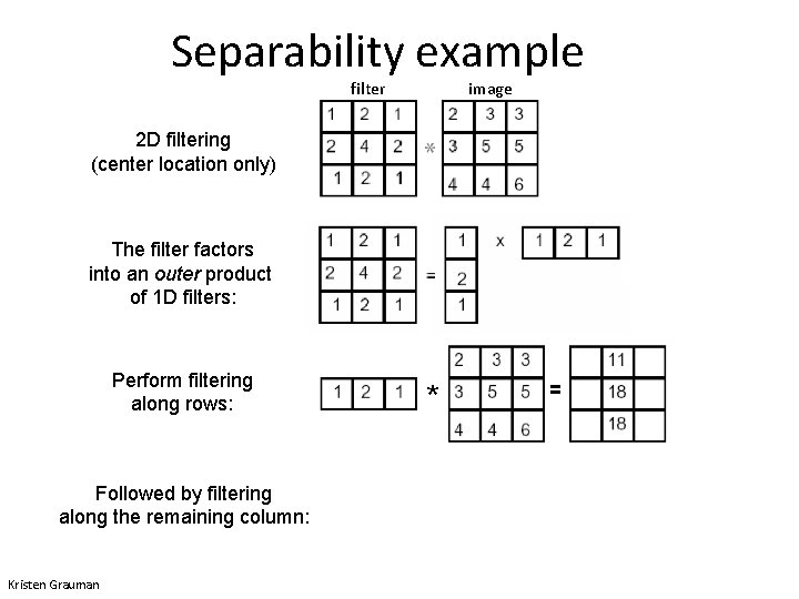
Separability example filter image 2 D filtering (center location only) The filter factors into an outer product of 1 D filters: Perform filtering along rows: Followed by filtering along the remaining column: Kristen Grauman * =

Plan for today • Feature detection / keypoint extraction – Corner detection – Blob detection • Start: Feature description (of detected features)

Problems with pixel representation • Not invariant to small changes – Translation – Illumination – etc. • Some parts of an image are more important than others • What do we want to represent?

Local features • Local means that they only cover a small part of the image • There will be many local features detected in an image • Later we’ll talk about how to use those to compute a representation of the whole image • Local features usually exploit image gradients, rarely color (we’ll revisit this statement with CNNs)

Local features: desired properties • Locality – A feature occupies a relatively small area of the image; robust to clutter and occlusion • Repeatability and flexibility – The same feature can be found in several images despite geometric, photometric transformations – Robustness to expected variations – Maximize correct matches • Distinctiveness – Each feature has a distinctive description – Minimize wrong matches • Compactness and efficiency – Many fewer features than image pixels Adapted from K. Grauman and D. Hoiem

Interest(ing) points • Note: “interest points” = “keypoints”, also sometimes called “features” • Many applications – Image search: which points would allow us to match images between query and database? – Recognition: which patches are likely to tell us something about object category? – 3 D reconstruction: how to find correspondences across different views? – Tracking: which points are good to track? Adapted from D. Hoiem

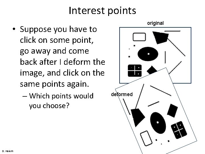
Interest points original • Suppose you have to click on some point, go away and come back after I deform the image, and click on the same points again. – Which points would you choose? D. Hoiem deformed

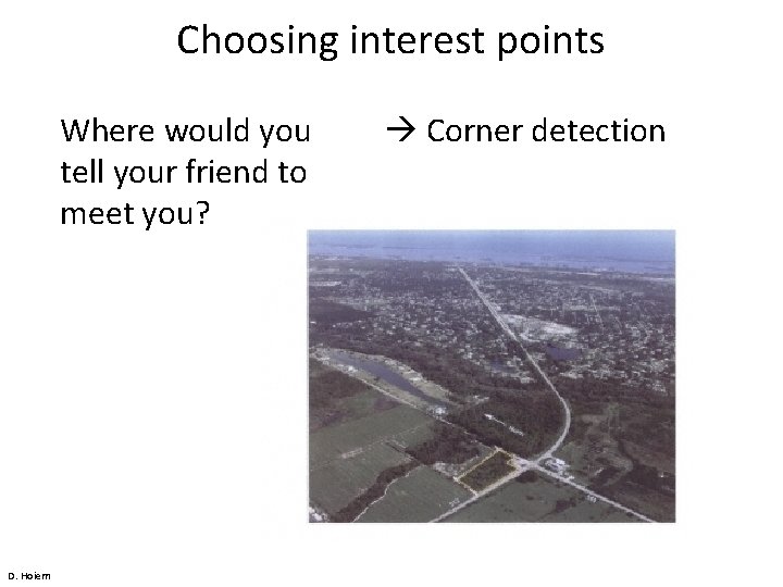
Choosing interest points Where would you tell your friend to meet you? D. Hoiem Corner detection

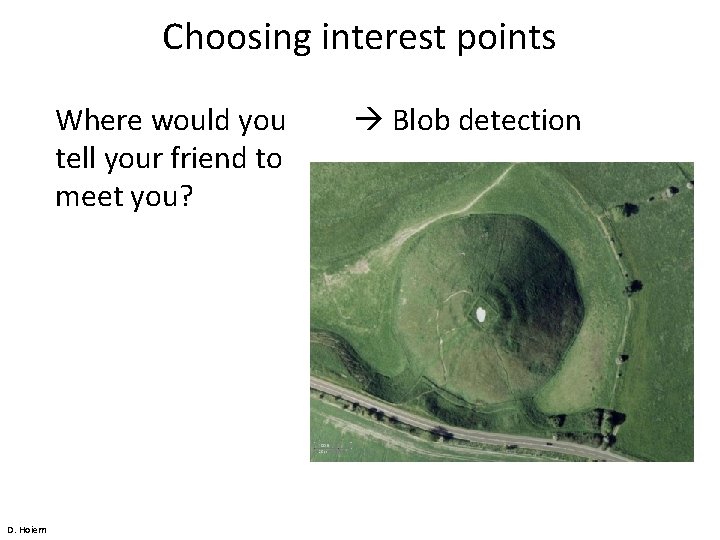
Choosing interest points Where would you tell your friend to meet you? D. Hoiem Blob detection

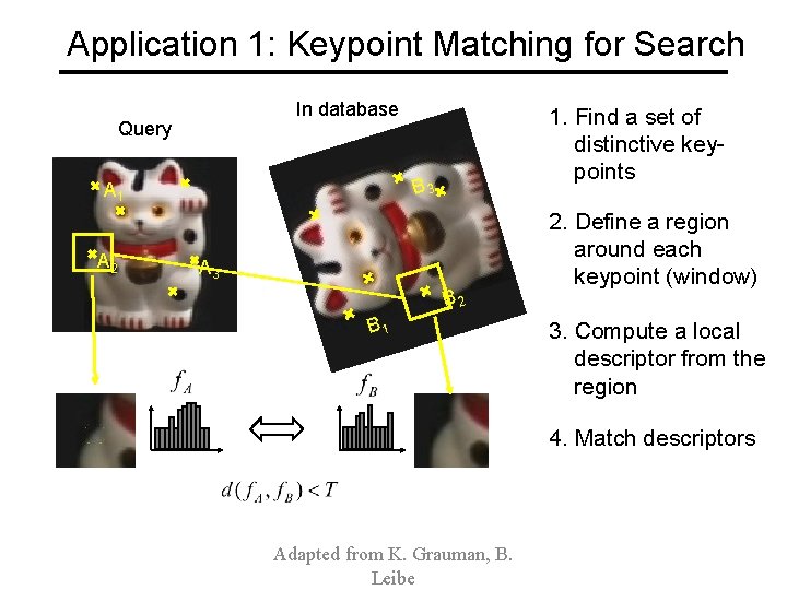
Application 1: Keypoint Matching for Search In database Query B 3 A 1 A 2 1. Find a set of distinctive keypoints A 3 B 2 B 1 2. Define a region around each keypoint (window) 3. Compute a local descriptor from the region 4. Match descriptors Adapted from K. Grauman, B. Leibe

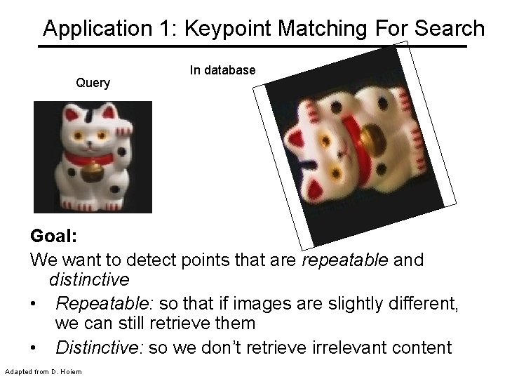
Application 1: Keypoint Matching For Search Query In database Goal: We want to detect points that are repeatable and distinctive • Repeatable: so that if images are slightly different, we can still retrieve them • Distinctive: so we don’t retrieve irrelevant content Adapted from D. Hoiem

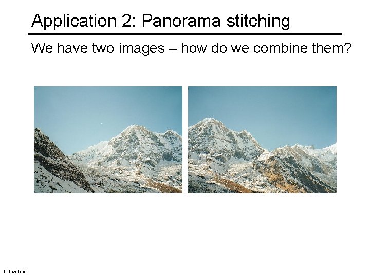
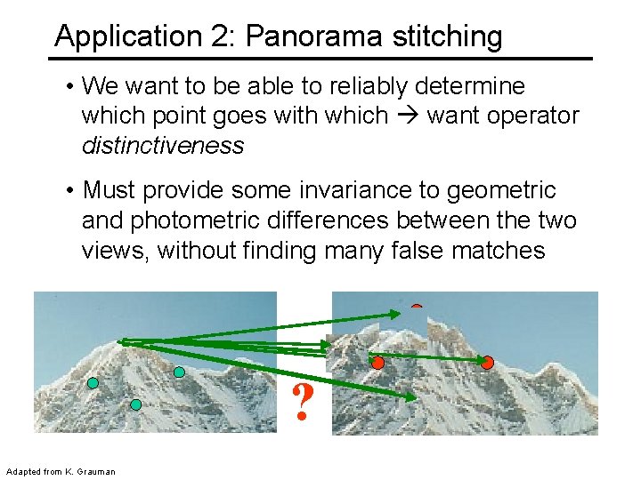
Application 2: Panorama stitching We have two images – how do we combine them? L. Lazebnik

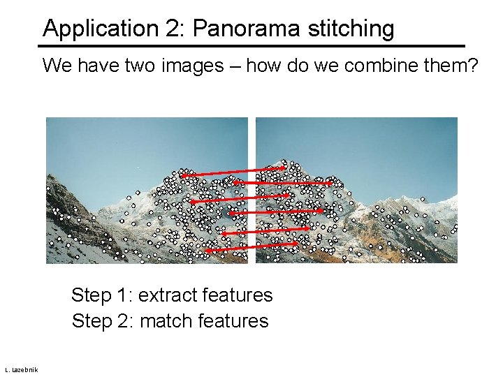
Application 2: Panorama stitching We have two images – how do we combine them? Step 1: extract features Step 2: match features L. Lazebnik

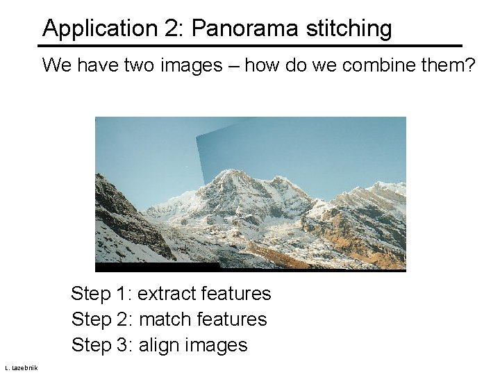
Application 2: Panorama stitching We have two images – how do we combine them? Step 1: extract features Step 2: match features Step 3: align images L. Lazebnik

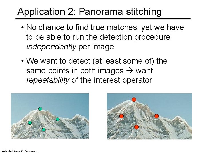
Application 2: Panorama stitching • No chance to find true matches, yet we have to be able to run the detection procedure independently per image. • We want to detect (at least some of) the same points in both images want repeatability of the interest operator Adapted from K. Grauman

Application 2: Panorama stitching • We want to be able to reliably determine which point goes with which want operator distinctiveness • Must provide some invariance to geometric and photometric differences between the two views, without finding many false matches ? Adapted from K. Grauman

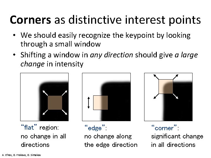
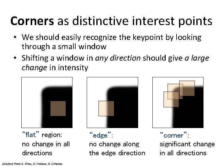
Corners as distinctive interest points • We should easily recognize the keypoint by looking through a small window • Shifting a window in any direction should give a large change in intensity “flat” region: no change in all directions A. Efros, D. Frolova, D. Simakov “edge”: no change along the edge direction “corner”: significant change in all directions

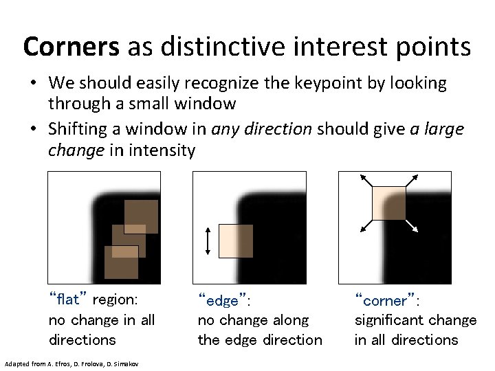
Corners as distinctive interest points • We should easily recognize the keypoint by looking through a small window • Shifting a window in any direction should give a large change in intensity “flat” region: no change in all directions Adapted from A. Efros, D. Frolova, D. Simakov “edge”: no change along the edge direction “corner”: significant change in all directions

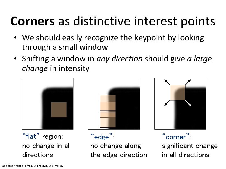
Corners as distinctive interest points • We should easily recognize the keypoint by looking through a small window • Shifting a window in any direction should give a large change in intensity “flat” region: no change in all directions Adapted from A. Efros, D. Frolova, D. Simakov “edge”: no change along the edge direction “corner”: significant change in all directions

Corners as distinctive interest points • We should easily recognize the keypoint by looking through a small window • Shifting a window in any direction should give a large change in intensity “flat” region: no change in all directions Adapted from A. Efros, D. Frolova, D. Simakov “edge”: no change along the edge direction “corner”: significant change in all directions

Corners as distinctive interest points • We should easily recognize the keypoint by looking through a small window • Shifting a window in any direction should give a large change in intensity “flat” region: no change in all directions Adapted from A. Efros, D. Frolova, D. Simakov “edge”: no change along the edge direction “corner”: significant change in all directions

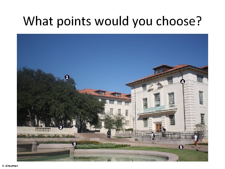
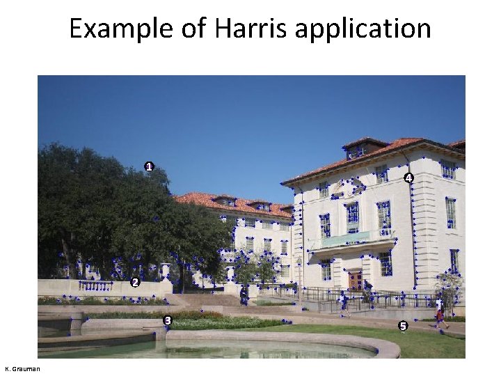
What points would you choose? 1 4 2 3 K. Grauman 5

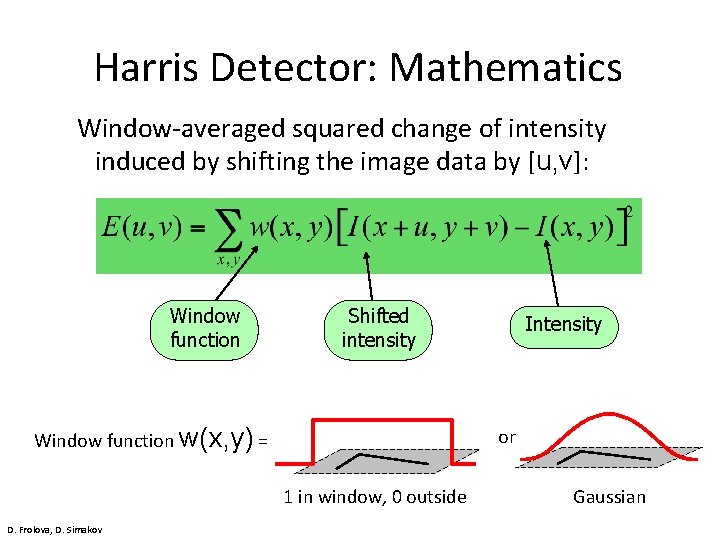
Harris Detector: Mathematics Window-averaged squared change of intensity induced by shifting the image data by [u, v]: Window function Shifted intensity Window function w(x, y) = or 1 in window, 0 outside D. Frolova, D. Simakov Intensity Gaussian

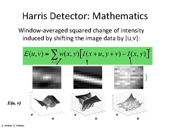
Harris Detector: Mathematics Window-averaged squared change of intensity induced by shifting the image data by [u, v]: Window function Shifted intensity Intensity E(u, v) v D. Frolova, D. Simakov u v u

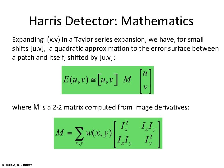
Harris Detector: Mathematics Expanding I(x, y) in a Taylor series expansion, we have, for small shifts [u, v], a quadratic approximation to the error surface between a patch and itself, shifted by [u, v]: where M is a 2× 2 matrix computed from image derivatives: D. Frolova, D. Simakov

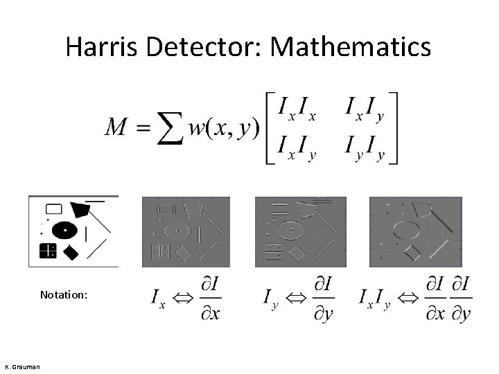
Harris Detector: Mathematics Notation: K. Grauman

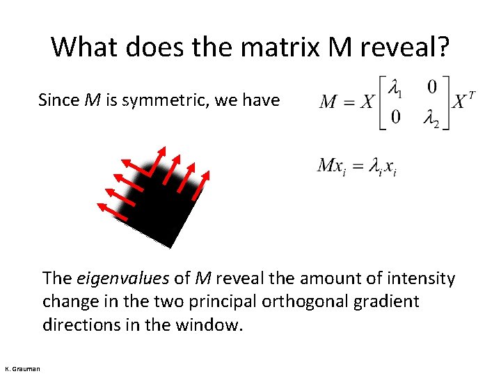
What does the matrix M reveal? Since M is symmetric, we have The eigenvalues of M reveal the amount of intensity change in the two principal orthogonal gradient directions in the window. K. Grauman

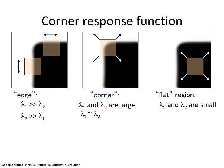
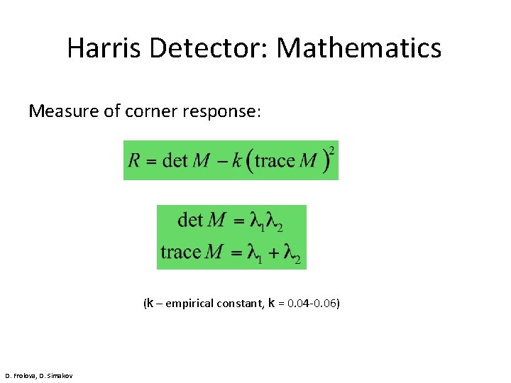
Corner response function “edge”: 1 >> 2 2 >> 1 “corner”: 1 and 2 are large, 1 ~ 2 Adapted from A. Efros, D. Frolova, D. Simakov, K. Grauman “flat” region: 1 and 2 are small

Harris Detector: Mathematics Measure of corner response: (k – empirical constant, k = 0. 04 -0. 06) D. Frolova, D. Simakov

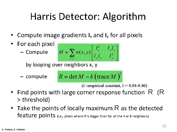
Harris Detector: Algorithm • Compute image gradients Ix and Iy for all pixels • For each pixel – Compute by looping over neighbors x, y – compute (k : empirical constant, k = 0. 04 -0. 06) • Find points with large corner response function R (R > threshold) • Take the points of locally maximum R as the detected feature points (i. e. , pixels where R is bigger than for all the 4 or 8 neighbors) D. Frolova, D. Simakov 35

Example of Harris application 1 4 2 3 K. Grauman 5

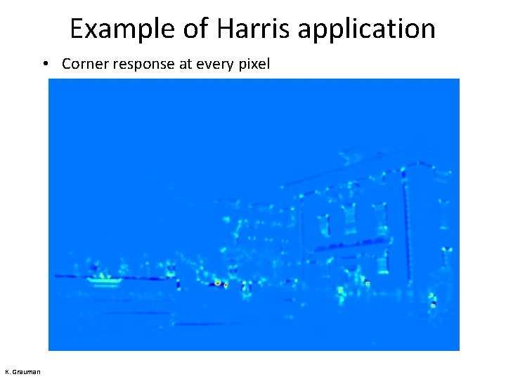
Example of Harris application • Corner response at every pixel K. Grauman

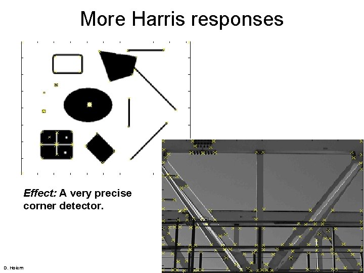
More Harris responses Effect: A very precise corner detector. D. Hoiem

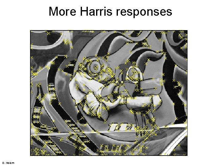
More Harris responses D. Hoiem