CS 1674 Intro to Computer Vision Support Vector

CS 1674: Intro to Computer Vision Support Vector Machines Prof. Adriana Kovashka University of Pittsburgh October 31, 2016

Plan for today • Support vector machines – Separable case / non-separable case – Linear / non-linear (kernels) • The importance of generalization – The bias-variance trade-off (applies to all classifiers)

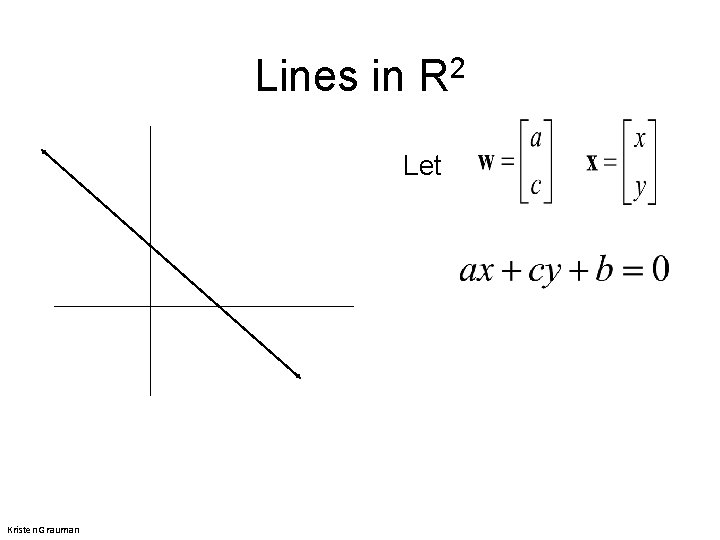
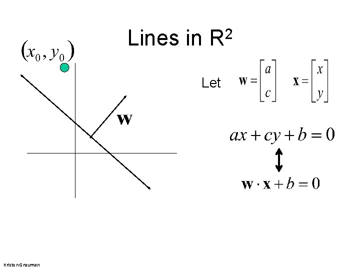
Lines in R 2 Let Kristen Grauman

Lines in R 2 Let Kristen Grauman

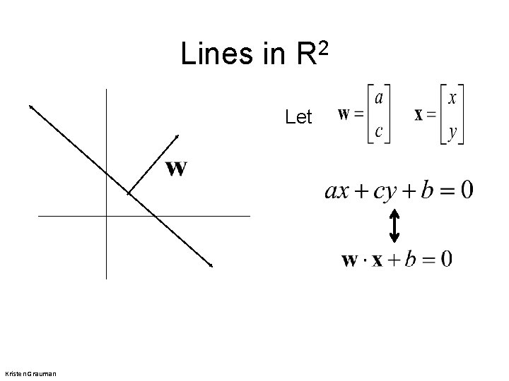
Lines in R 2 Let Kristen Grauman

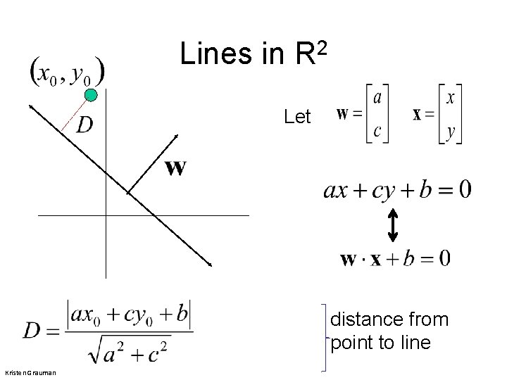
Lines in R 2 Let distance from point to line Kristen Grauman

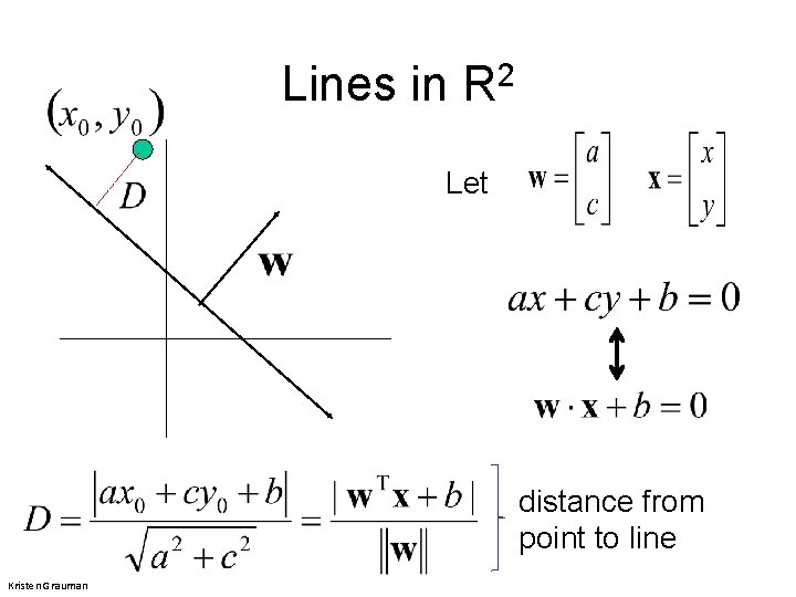
Lines in R 2 Let distance from point to line Kristen Grauman

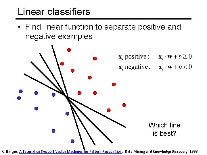
Linear classifiers • Find linear function to separate positive and negative examples Which line is best? C. Burges, A Tutorial on Support Vector Machines for Pattern Recognition, Data Mining and Knowledge Discovery, 1998

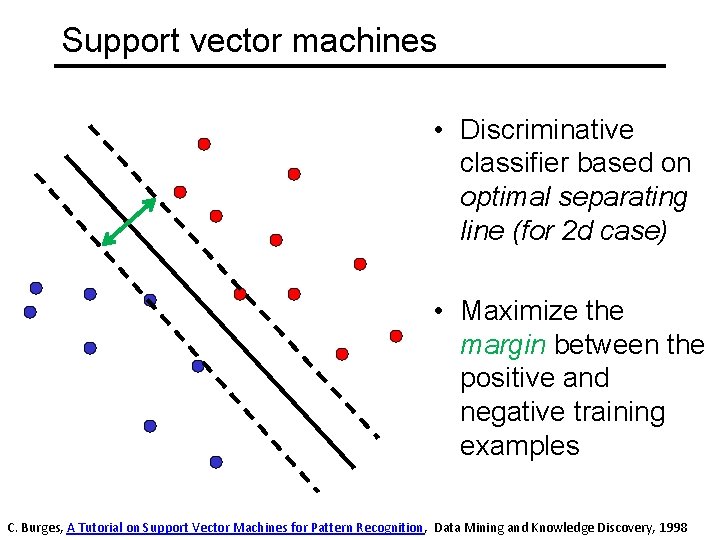
Support vector machines • Discriminative classifier based on optimal separating line (for 2 d case) • Maximize the margin between the positive and negative training examples C. Burges, A Tutorial on Support Vector Machines for Pattern Recognition, Data Mining and Knowledge Discovery, 1998

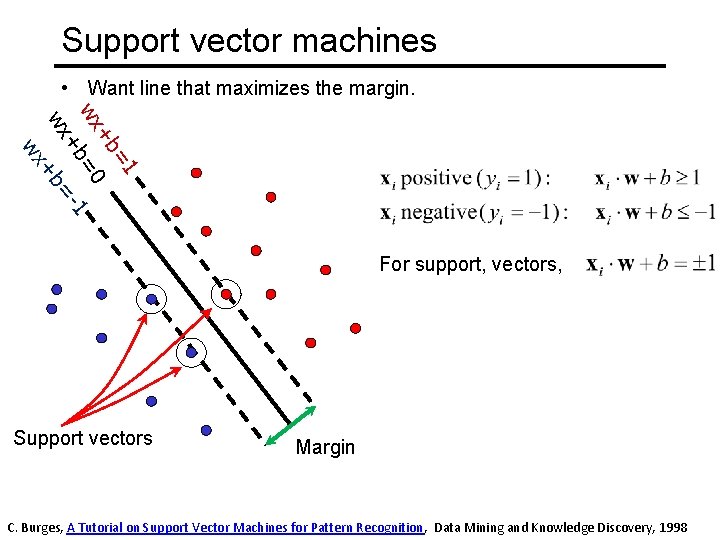
Support vector machines • Want line that maximizes the margin. =1 +b wx =0 1 +b wx +b= wx For support, vectors, Support vectors Margin C. Burges, A Tutorial on Support Vector Machines for Pattern Recognition, Data Mining and Knowledge Discovery, 1998

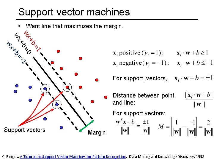
Support vector machines • Want line that maximizes the margin. =1 +b wx =0 1 +b wx +b= wx For support, vectors, Distance between point and line: For support vectors: Support vectors Margin C. Burges, A Tutorial on Support Vector Machines for Pattern Recognition, Data Mining and Knowledge Discovery, 1998

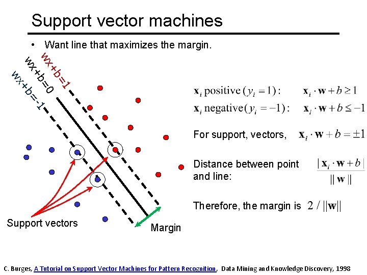
Support vector machines • Want line that maximizes the margin. =1 +b wx =0 1 +b wx +b= wx For support, vectors, Distance between point and line: Therefore, the margin is Support vectors 2 / ||w|| Margin C. Burges, A Tutorial on Support Vector Machines for Pattern Recognition, Data Mining and Knowledge Discovery, 1998

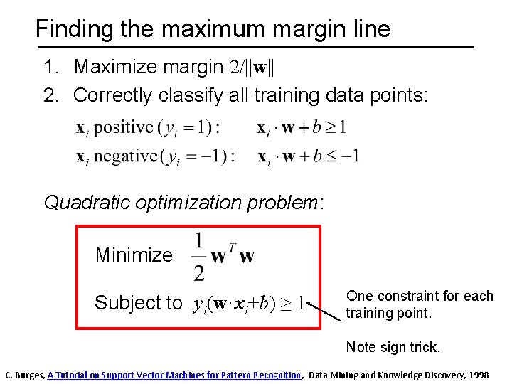
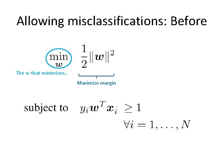
Finding the maximum margin line 1. Maximize margin 2/||w|| 2. Correctly classify all training data points: Quadratic optimization problem: Minimize Subject to yi(w·xi+b) ≥ 1 One constraint for each training point. Note sign trick. C. Burges, A Tutorial on Support Vector Machines for Pattern Recognition, Data Mining and Knowledge Discovery, 1998

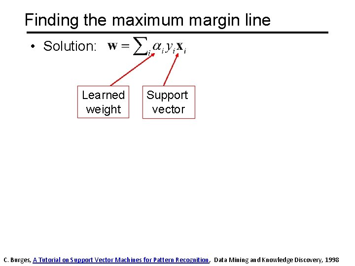
Finding the maximum margin line • Solution: Learned weight Support vector C. Burges, A Tutorial on Support Vector Machines for Pattern Recognition, Data Mining and Knowledge Discovery, 1998

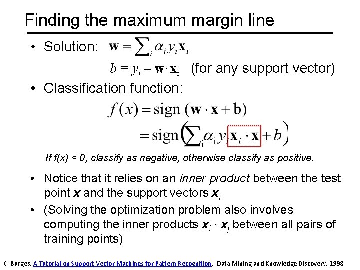
Finding the maximum margin line • Solution: b = yi – w·xi (for any support vector) • Classification function: If f(x) < 0, classify as negative, otherwise classify as positive. • Notice that it relies on an inner product between the test point x and the support vectors xi • (Solving the optimization problem also involves computing the inner products xi · xj between all pairs of training points) C. Burges, A Tutorial on Support Vector Machines for Pattern Recognition, Data Mining and Knowledge Discovery, 1998

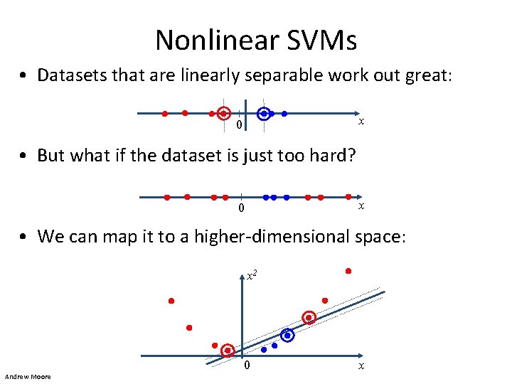
Nonlinear SVMs • Datasets that are linearly separable work out great: x 0 • But what if the dataset is just too hard? x 0 • We can map it to a higher-dimensional space: x 2 0 Andrew Moore x

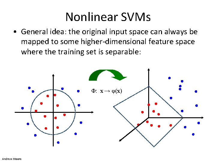
Nonlinear SVMs • General idea: the original input space can always be mapped to some higher-dimensional feature space where the training set is separable: Φ: x → φ(x) Andrew Moore

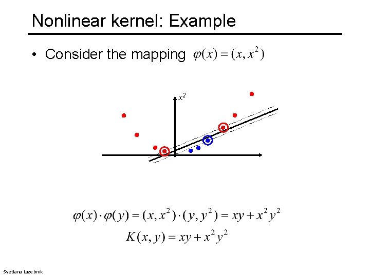
Nonlinear kernel: Example • Consider the mapping x 2 Svetlana Lazebnik

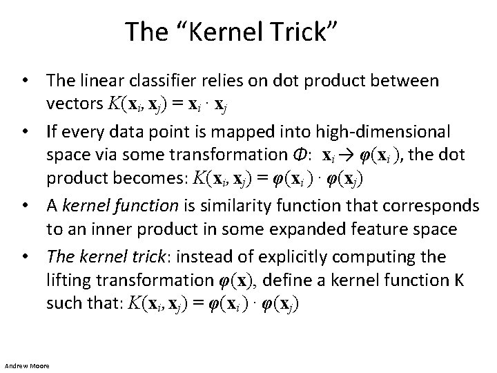
The “Kernel Trick” • The linear classifier relies on dot product between vectors K(xi , xj) = xi · xj • If every data point is mapped into high-dimensional space via some transformation Φ: xi → φ(xi ), the dot product becomes: K(xi , xj) = φ(xi ) · φ(xj) • A kernel function is similarity function that corresponds to an inner product in some expanded feature space • The kernel trick: instead of explicitly computing the lifting transformation φ(x), define a kernel function K such that: K(xi , xj) = φ(xi ) · φ(xj) Andrew Moore

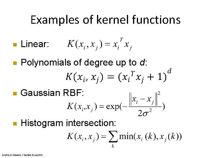
Examples of kernel functions n Linear: n Polynomials of degree up to d: n Gaussian RBF: n Histogram intersection: Andrew Moore / Carlos Guestrin

Allowing misclassifications: Before The w that minimizes… Maximize margin

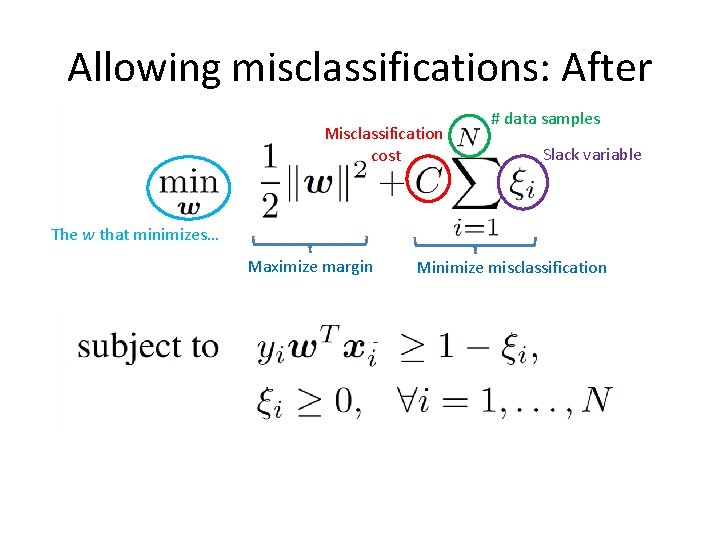
Allowing misclassifications: After Misclassification cost # data samples Slack variable The w that minimizes… Maximize margin Minimize misclassification

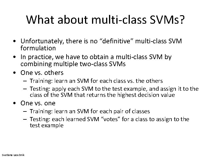
What about multi-class SVMs? • Unfortunately, there is no “definitive” multi-class SVM formulation • In practice, we have to obtain a multi-class SVM by combining multiple two-class SVMs • One vs. others – Training: learn an SVM for each class vs. the others – Testing: apply each SVM to the test example, and assign it to the class of the SVM that returns the highest decision value • One vs. one – Training: learn an SVM for each pair of classes – Testing: each learned SVM “votes” for a class to assign to the test example Svetlana Lazebnik

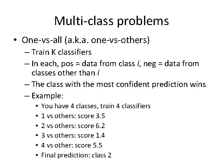
Multi-class problems • One-vs-all (a. k. a. one-vs-others) – Train K classifiers – In each, pos = data from class i, neg = data from classes other than i – The class with the most confident prediction wins – Example: • • • You have 4 classes, train 4 classifiers 1 vs others: score 3. 5 2 vs others: score 6. 2 3 vs others: score 1. 4 4 vs other: score 5. 5 Final prediction: class 2

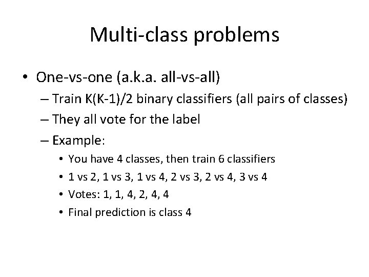
Multi-class problems • One-vs-one (a. k. a. all-vs-all) – Train K(K-1)/2 binary classifiers (all pairs of classes) – They all vote for the label – Example: • • You have 4 classes, then train 6 classifiers 1 vs 2, 1 vs 3, 1 vs 4, 2 vs 3, 2 vs 4, 3 vs 4 Votes: 1, 1, 4, 2, 4, 4 Final prediction is class 4

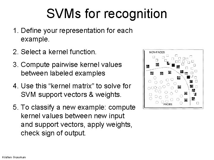
SVMs for recognition 1. Define your representation for each example. 2. Select a kernel function. 3. Compute pairwise kernel values between labeled examples 4. Use this “kernel matrix” to solve for SVM support vectors & weights. 5. To classify a new example: compute kernel values between new input and support vectors, apply weights, check sign of output. Kristen Grauman

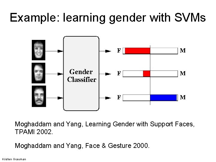
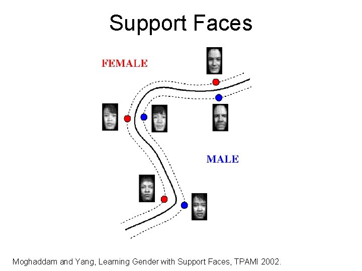
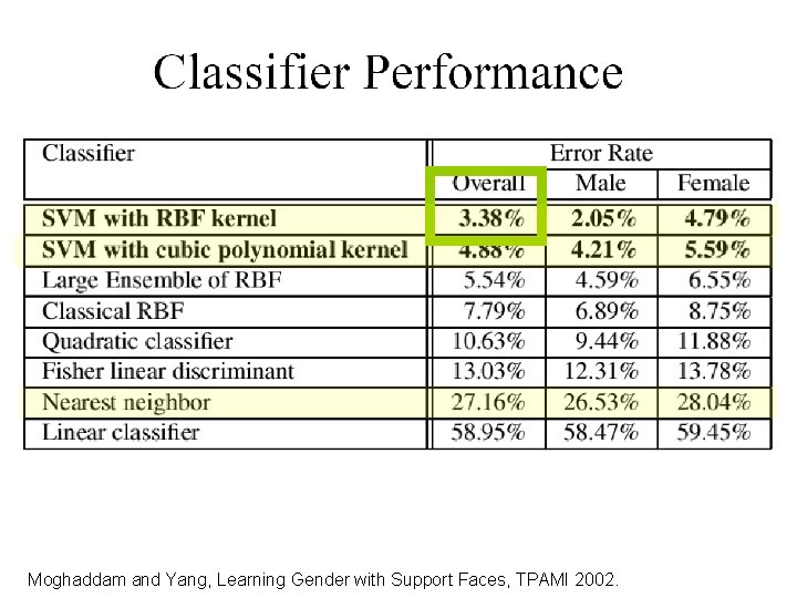
Example: learning gender with SVMs Moghaddam and Yang, Learning Gender with Support Faces, TPAMI 2002. Moghaddam and Yang, Face & Gesture 2000. Kristen Grauman

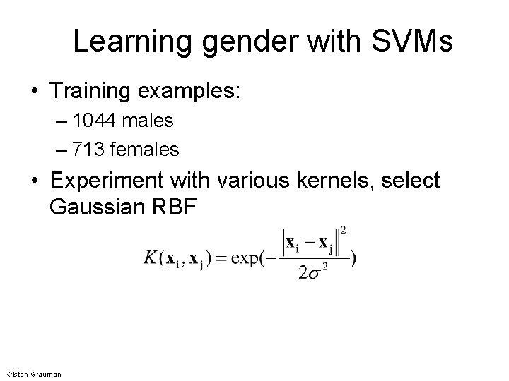
Learning gender with SVMs • Training examples: – 1044 males – 713 females • Experiment with various kernels, select Gaussian RBF Kristen Grauman

Support Faces Moghaddam and Yang, Learning Gender with Support Faces, TPAMI 2002.

Moghaddam and Yang, Learning Gender with Support Faces, TPAMI 2002.

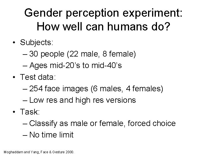
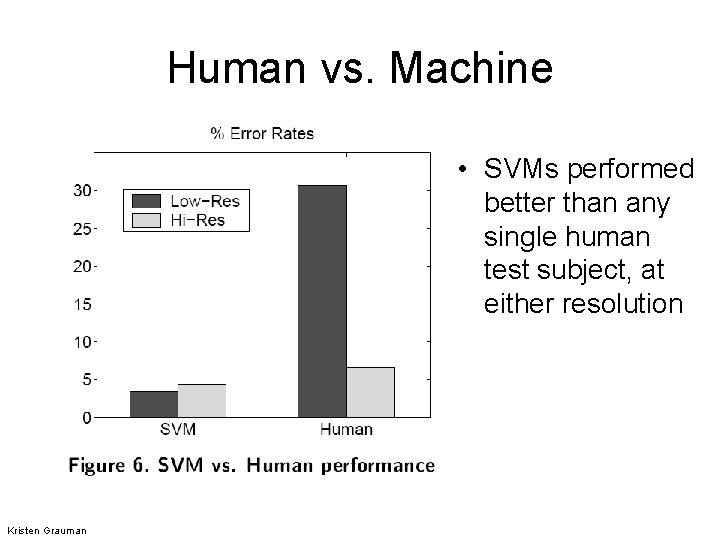
Gender perception experiment: How well can humans do? • Subjects: – 30 people (22 male, 8 female) – Ages mid-20’s to mid-40’s • Test data: – 254 face images (6 males, 4 females) – Low res and high res versions • Task: – Classify as male or female, forced choice – No time limit Moghaddam and Yang, Face & Gesture 2000.

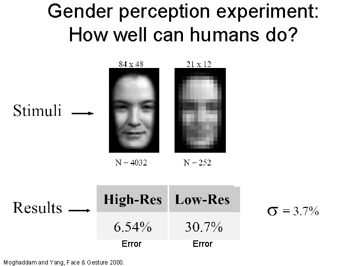
Gender perception experiment: How well can humans do? Error Moghaddam and Yang, Face & Gesture 2000. Error

Human vs. Machine • SVMs performed better than any single human test subject, at either resolution Kristen Grauman

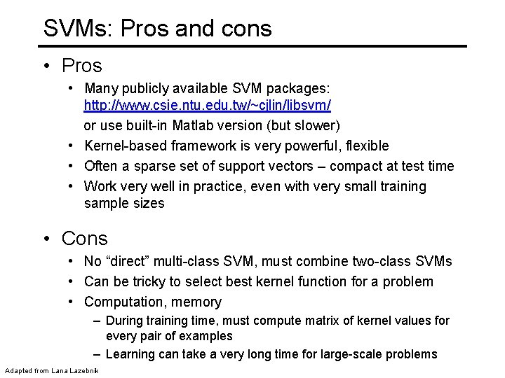
SVMs: Pros and cons • Pros • Many publicly available SVM packages: http: //www. csie. ntu. edu. tw/~cjlin/libsvm/ or use built-in Matlab version (but slower) • Kernel-based framework is very powerful, flexible • Often a sparse set of support vectors – compact at test time • Work very well in practice, even with very small training sample sizes • Cons • No “direct” multi-class SVM, must combine two-class SVMs • Can be tricky to select best kernel function for a problem • Computation, memory – During training time, must compute matrix of kernel values for every pair of examples – Learning can take a very long time for large-scale problems Adapted from Lana Lazebnik

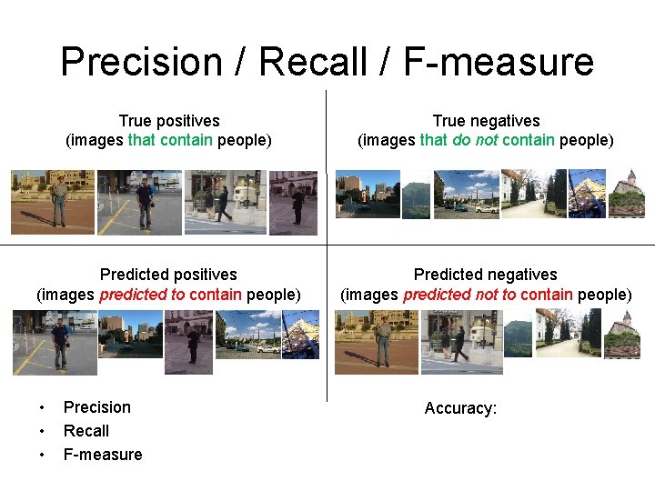
Precision / Recall / F-measure True positives (images that contain people) True negatives (images that do not contain people) Predicted positives (images predicted to contain people) Predicted negatives (images predicted not to contain people) • • • Precision Recall F-measure = 2 / 5 = 0. 4 = 2 / 4 = 0. 5 = 2*0. 4*0. 5 / 0. 4+0. 5 = 0. 44 Accuracy: 5 / 10 = 0. 5

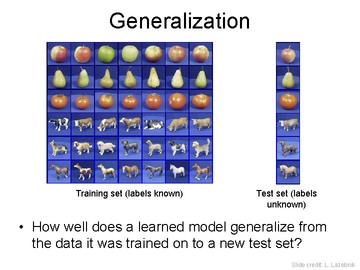
Generalization Training set (labels known) Test set (labels unknown) • How well does a learned model generalize from the data it was trained on to a new test set? Slide credit: L. Lazebnik

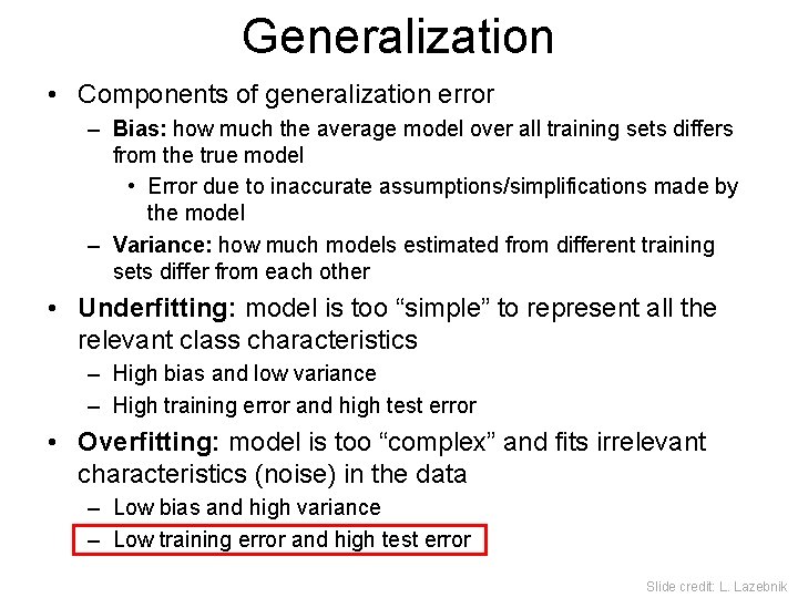
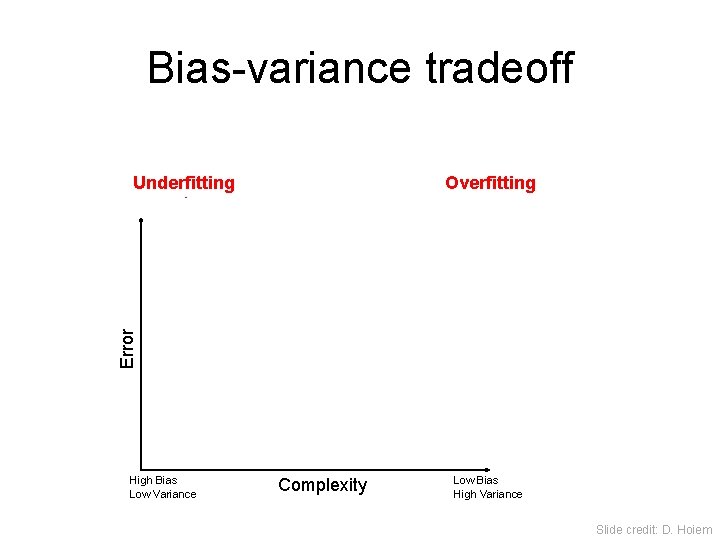
Generalization • Components of generalization error – Bias: how much the average model over all training sets differs from the true model • Error due to inaccurate assumptions/simplifications made by the model – Variance: how much models estimated from different training sets differ from each other • Underfitting: model is too “simple” to represent all the relevant class characteristics – High bias and low variance – High training error and high test error • Overfitting: model is too “complex” and fits irrelevant characteristics (noise) in the data – Low bias and high variance – Low training error and high test error Slide credit: L. Lazebnik

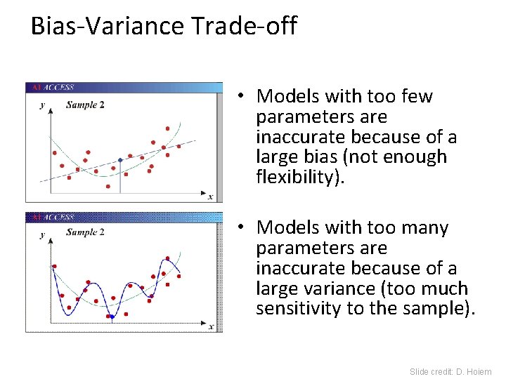
Bias-Variance Trade-off • Models with too few parameters are inaccurate because of a large bias (not enough flexibility). • Models with too many parameters are inaccurate because of a large variance (too much sensitivity to the sample). Slide credit: D. Hoiem

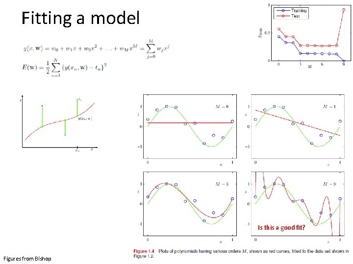
Fitting a model Is this a good fit? Figures from Bishop

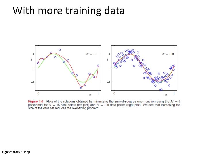
With more training data Figures from Bishop

Bias-variance tradeoff Overfitting Error Underfitting Test error Training error High Bias Low Variance Complexity Low Bias High Variance Slide credit: D. Hoiem

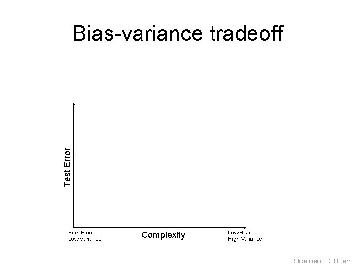
Bias-variance tradeoff Test Error Few training examples High Bias Low Variance Many training examples Complexity Low Bias High Variance Slide credit: D. Hoiem

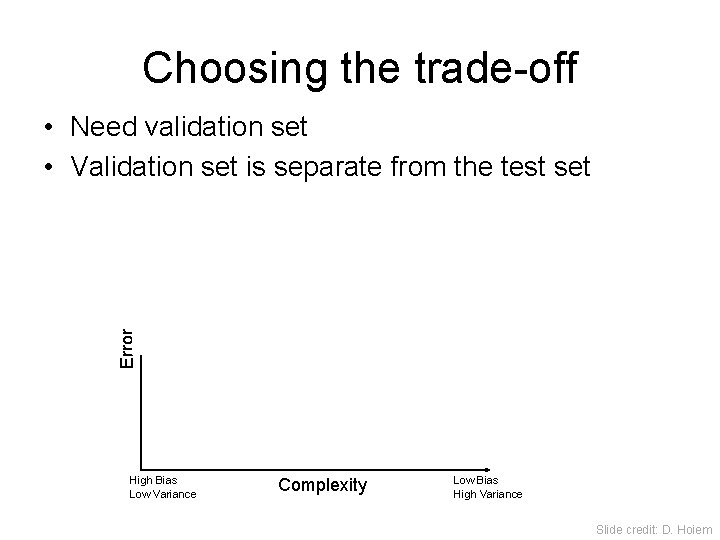
Choosing the trade-off • Need validation set • Validation set is separate from the test set Error Validation error Training error High Bias Low Variance Complexity Low Bias High Variance Slide credit: D. Hoiem

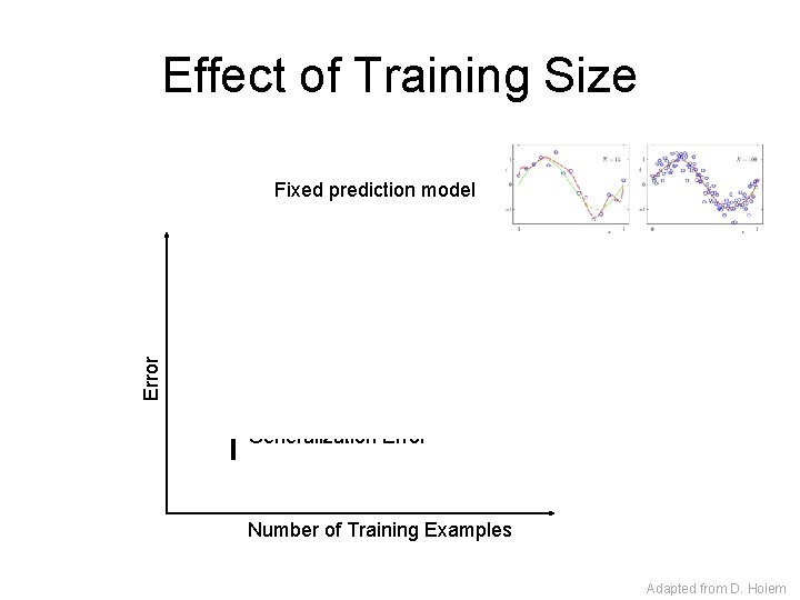
Effect of Training Size Error Fixed prediction model Testing Generalization Error Training Number of Training Examples Adapted from D. Hoiem

How to reduce variance? • Choose a simpler classifier • Use fewer features • Get more training data • Regularize the parameters Slide credit: D. Hoiem

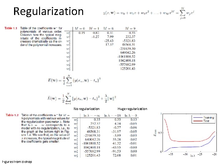
Regularization No regularization Figures from Bishop Huge regularization

Characteristics of vision learning problems • Lots of continuous features – Spatial pyramid may have ~15, 000 features • Imbalanced classes – Often limited positive examples, practically infinite negative examples • Difficult prediction tasks • Recently, massive training sets became available – If we have a massive training set, we want classifiers with low bias (high variance is ok) and reasonably efficient training Adapted from D. Hoiem

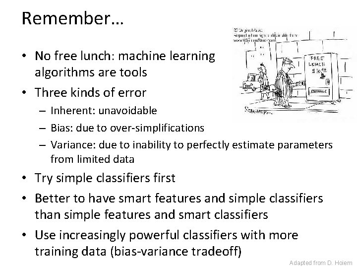
Remember… • No free lunch: machine learning algorithms are tools • Three kinds of error – Inherent: unavoidable – Bias: due to over-simplifications – Variance: due to inability to perfectly estimate parameters from limited data • Try simple classifiers first • Better to have smart features and simple classifiers than simple features and smart classifiers • Use increasingly powerful classifiers with more training data (bias-variance tradeoff) Adapted from D. Hoiem