CS 1699 Intro to Computer Vision Support Vector

CS 1699: Intro to Computer Vision Support Vector Machines Prof. Adriana Kovashka University of Pittsburgh October 29, 2015

Homework • HW 3: due Nov. 3 – Note: You need to perform k-means on features from multiple frames joined together, not one kmeans per frame! • HW 4: due Nov. 24 • HW 5: half-length, still 10% of grade, out Nov. 24, due Dec. 10

Plan for today • Support vector machines • Bias-variance tradeoff • Scene recognition: Spatial pyramid matching

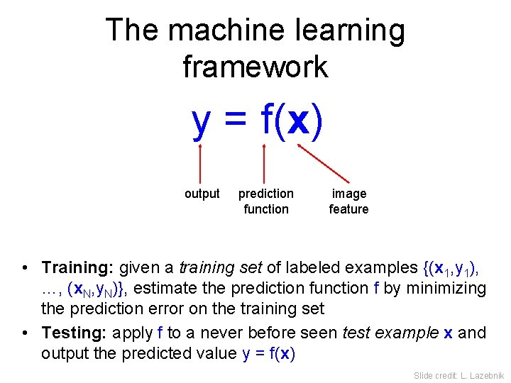
The machine learning framework y = f(x) output prediction function image feature • Training: given a training set of labeled examples {(x 1, y 1), …, (x. N, y. N)}, estimate the prediction function f by minimizing the prediction error on the training set • Testing: apply f to a never before seen test example x and output the predicted value y = f(x) Slide credit: L. Lazebnik

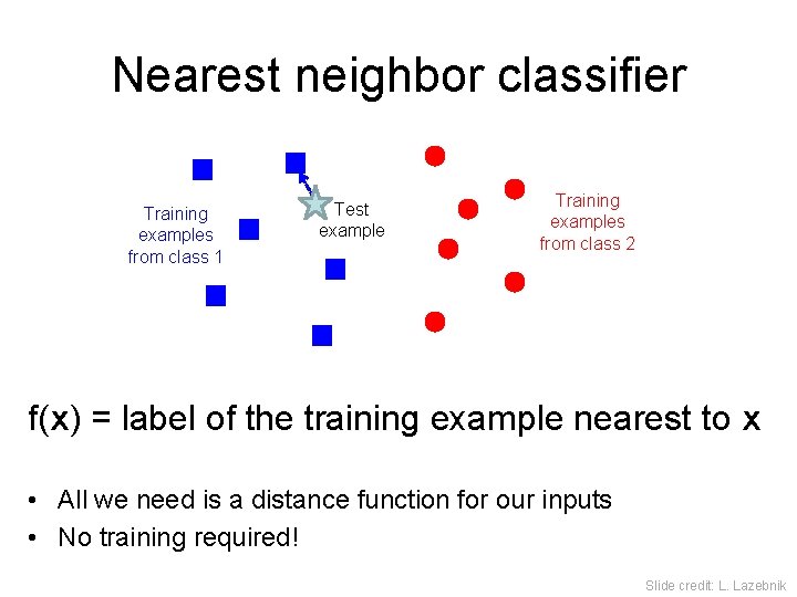
Nearest neighbor classifier Training examples from class 1 Test example Training examples from class 2 f(x) = label of the training example nearest to x • All we need is a distance function for our inputs • No training required! Slide credit: L. Lazebnik

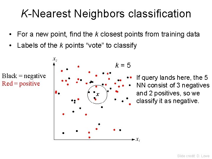
K-Nearest Neighbors classification • For a new point, find the k closest points from training data • Labels of the k points “vote” to classify k=5 Black = negative Red = positive If query lands here, the 5 NN consist of 3 negatives and 2 positives, so we classify it as negative. Slide credit: D. Lowe

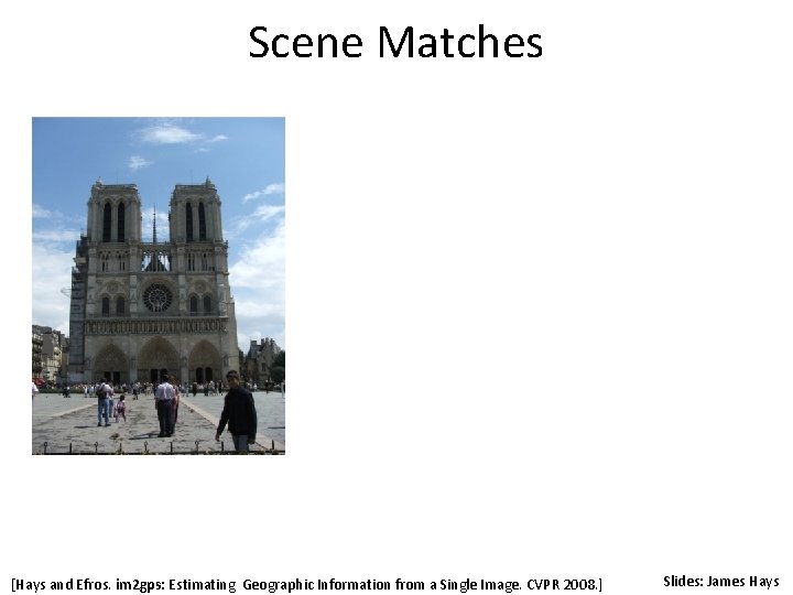
Scene Matches [Hays and Efros. im 2 gps: Estimating Geographic Information from a Single Image. CVPR 2008. ] Slides: James Hays

Nearest Neighbors: Pros and Cons • NN pros: + + Simple to implement Decision boundaries not necessarily linear Works for any number of classes Nonparametric method • NN cons: – Need good distance function – Slow at test time (large search problem to find neighbors) – Storage of data Adapted from L. Lazebnik

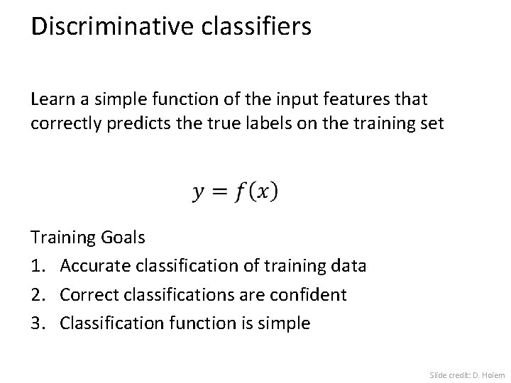
Discriminative classifiers Learn a simple function of the input features that correctly predicts the true labels on the training set Training Goals 1. Accurate classification of training data 2. Correct classifications are confident 3. Classification function is simple Slide credit: D. Hoiem

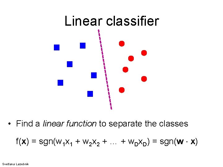
Linear classifier • Find a linear function to separate the classes f(x) = sgn(w 1 x 1 + w 2 x 2 + … + w. Dx. D) = sgn(w x) Svetlana Lazebnik

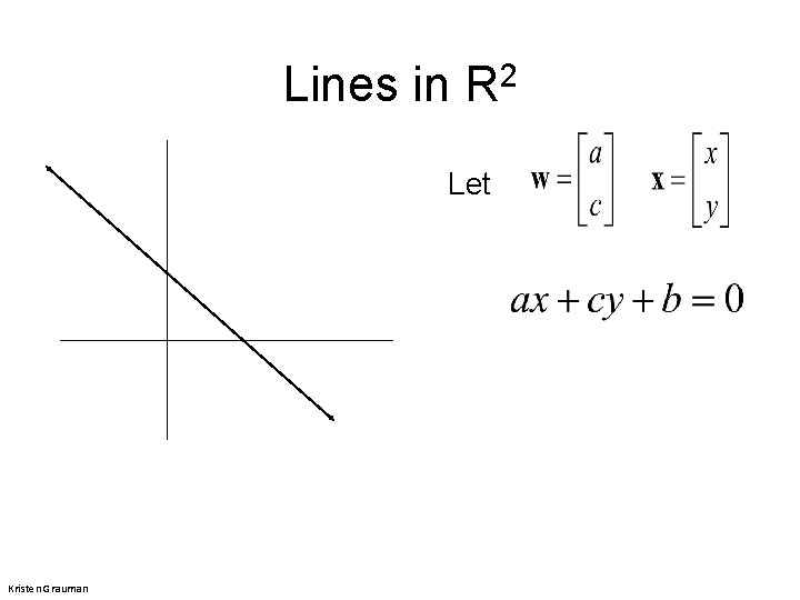
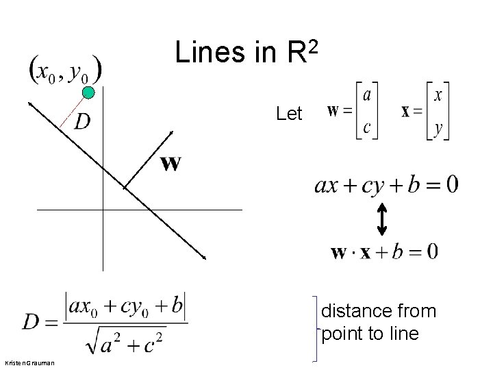
Lines in R 2 Let Kristen Grauman

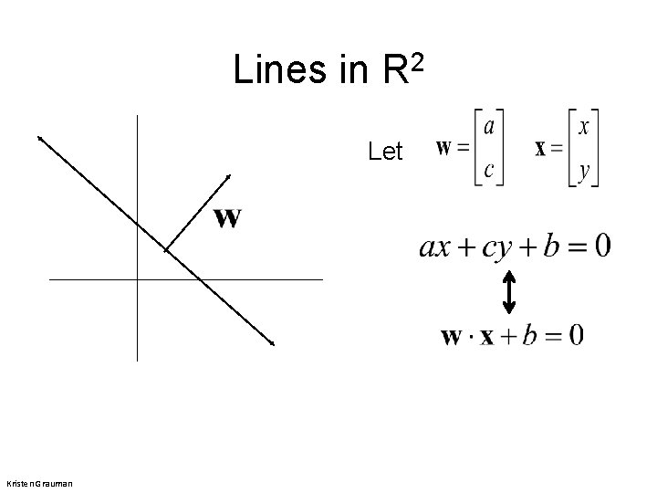
Lines in R 2 Let Kristen Grauman

Lines in R 2 Let Kristen Grauman

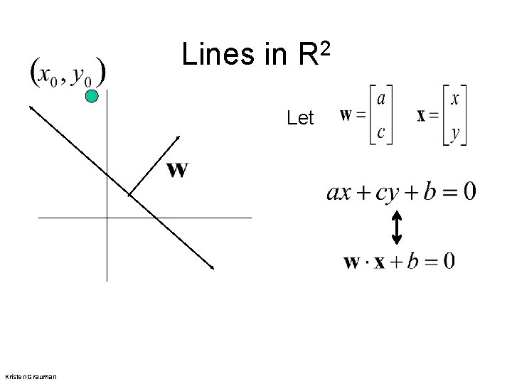
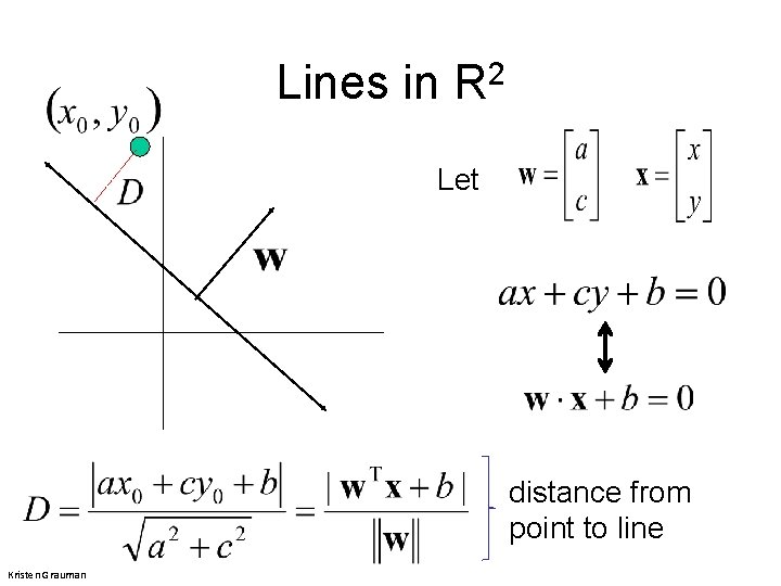
Lines in R 2 Let distance from point to line Kristen Grauman

Lines in R 2 Let distance from point to line Kristen Grauman

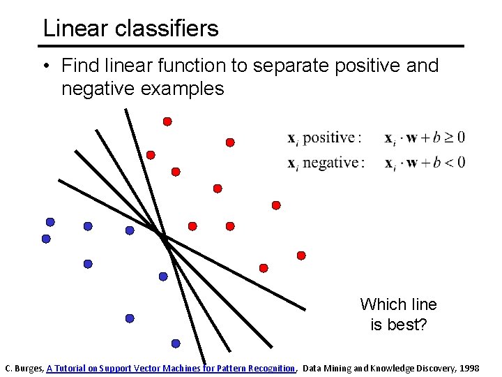
Linear classifiers • Find linear function to separate positive and negative examples Which line is best? C. Burges, A Tutorial on Support Vector Machines for Pattern Recognition, Data Mining and Knowledge Discovery, 1998

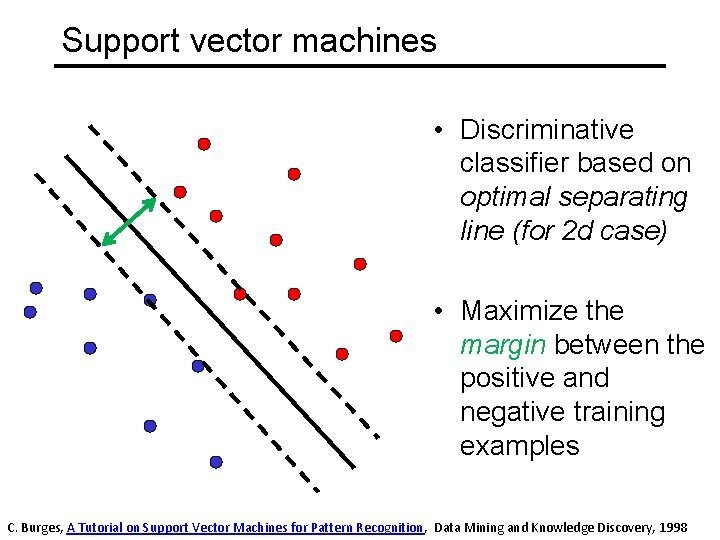
Support vector machines • Discriminative classifier based on optimal separating line (for 2 d case) • Maximize the margin between the positive and negative training examples C. Burges, A Tutorial on Support Vector Machines for Pattern Recognition, Data Mining and Knowledge Discovery, 1998

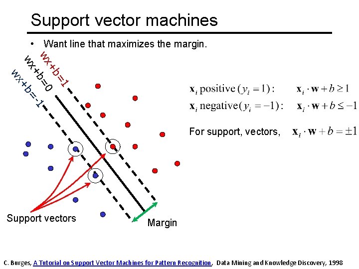
Support vector machines • Want line that maximizes the margin. =1 +b wx =0 1 +b wx +b= wx For support, vectors, Support vectors Margin C. Burges, A Tutorial on Support Vector Machines for Pattern Recognition, Data Mining and Knowledge Discovery, 1998

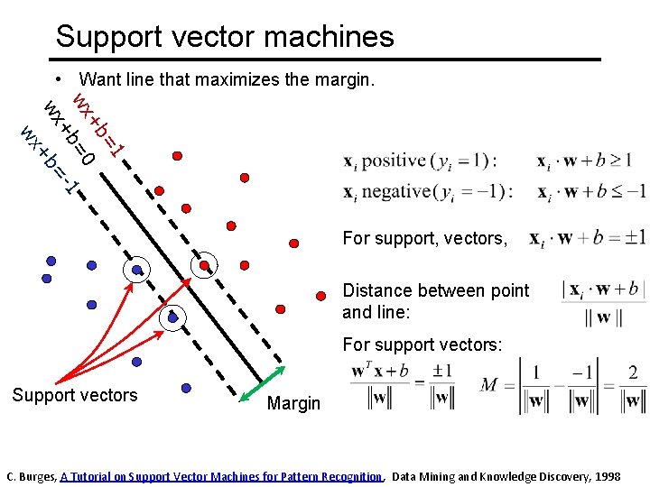
Support vector machines • Want line that maximizes the margin. =1 +b wx =0 1 +b wx +b= wx For support, vectors, Distance between point and line: For support vectors: Support vectors Margin C. Burges, A Tutorial on Support Vector Machines for Pattern Recognition, Data Mining and Knowledge Discovery, 1998

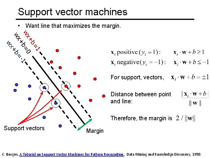
Support vector machines • Want line that maximizes the margin. =1 +b wx =0 1 +b wx +b= wx For support, vectors, Distance between point and line: Therefore, the margin is Support vectors 2 / ||w|| Margin C. Burges, A Tutorial on Support Vector Machines for Pattern Recognition, Data Mining and Knowledge Discovery, 1998

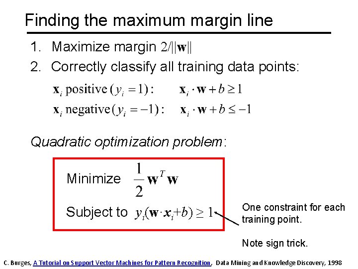
Finding the maximum margin line 1. Maximize margin 2/||w|| 2. Correctly classify all training data points: Quadratic optimization problem: Minimize Subject to yi(w·xi+b) ≥ 1 One constraint for each training point. Note sign trick. C. Burges, A Tutorial on Support Vector Machines for Pattern Recognition, Data Mining and Knowledge Discovery, 1998

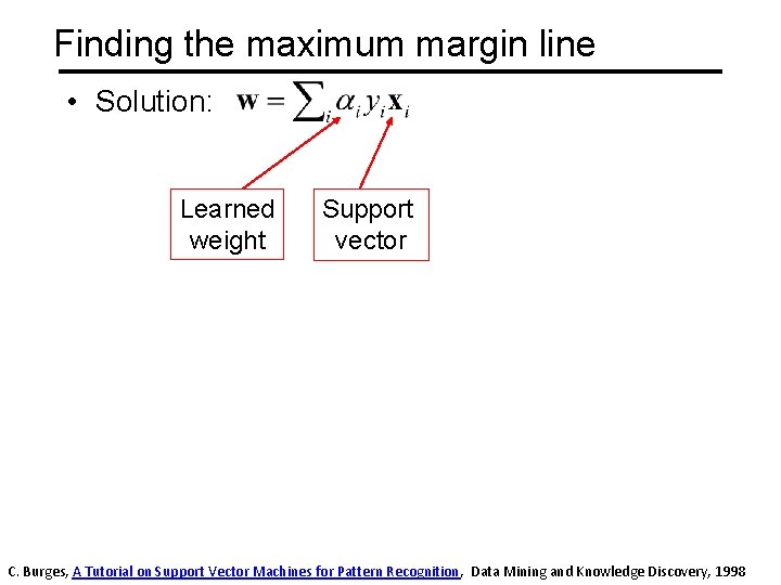
Finding the maximum margin line • Solution: Learned weight Support vector C. Burges, A Tutorial on Support Vector Machines for Pattern Recognition, Data Mining and Knowledge Discovery, 1998

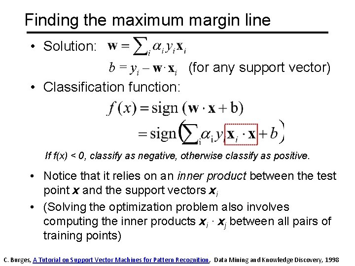
Finding the maximum margin line • Solution: b = yi – w·xi (for any support vector) • Classification function: If f(x) < 0, classify as negative, otherwise classify as positive. • Notice that it relies on an inner product between the test point x and the support vectors xi • (Solving the optimization problem also involves computing the inner products xi · xj between all pairs of training points) C. Burges, A Tutorial on Support Vector Machines for Pattern Recognition, Data Mining and Knowledge Discovery, 1998

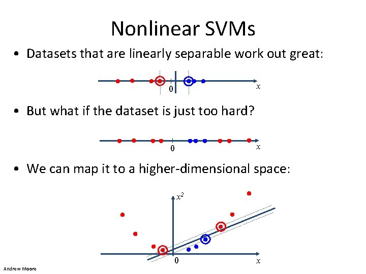
Nonlinear SVMs • Datasets that are linearly separable work out great: x 0 • But what if the dataset is just too hard? x 0 • We can map it to a higher-dimensional space: x 2 0 Andrew Moore x

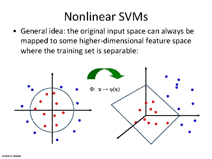
Nonlinear SVMs • General idea: the original input space can always be mapped to some higher-dimensional feature space where the training set is separable: Φ: x → φ(x) Andrew Moore

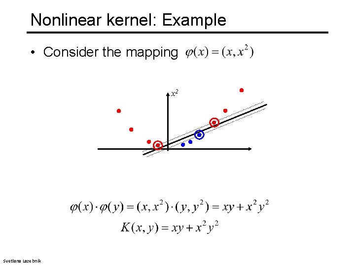
Nonlinear kernel: Example • Consider the mapping x 2 Svetlana Lazebnik

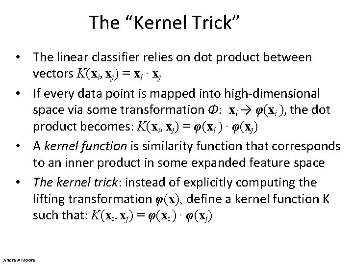
The “Kernel Trick” • The linear classifier relies on dot product between vectors K(xi , xj) = xi · xj • If every data point is mapped into high-dimensional space via some transformation Φ: xi → φ(xi ), the dot product becomes: K(xi , xj) = φ(xi ) · φ(xj) • A kernel function is similarity function that corresponds to an inner product in some expanded feature space • The kernel trick: instead of explicitly computing the lifting transformation φ(x), define a kernel function K such that: K(xi , xj) = φ(xi ) · φ(xj) Andrew Moore

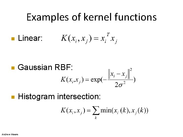
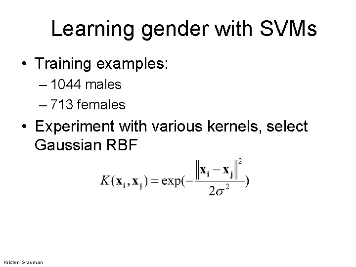
Examples of kernel functions n Linear: n Gaussian RBF: n Histogram intersection: Andrew Moore

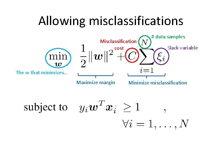
Allowing misclassifications Misclassification cost # data samples Slack variable The w that minimizes… Maximize margin Minimize misclassification

What about multi-class SVMs? • Unfortunately, there is no “definitive” multi-class SVM formulation • In practice, we have to obtain a multi-class SVM by combining multiple two-class SVMs • One vs. others – Training: learn an SVM for each class vs. the others – Testing: apply each SVM to the test example, and assign it to the class of the SVM that returns the highest decision value • One vs. one – Training: learn an SVM for each pair of classes – Testing: each learned SVM “votes” for a class to assign to the test example Svetlana Lazebnik

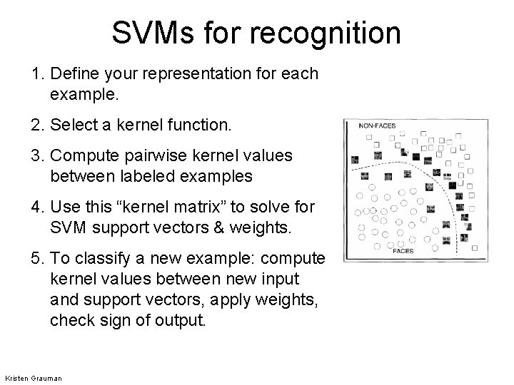
SVMs for recognition 1. Define your representation for each example. 2. Select a kernel function. 3. Compute pairwise kernel values between labeled examples 4. Use this “kernel matrix” to solve for SVM support vectors & weights. 5. To classify a new example: compute kernel values between new input and support vectors, apply weights, check sign of output. Kristen Grauman

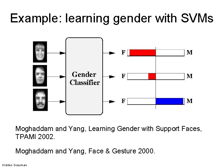
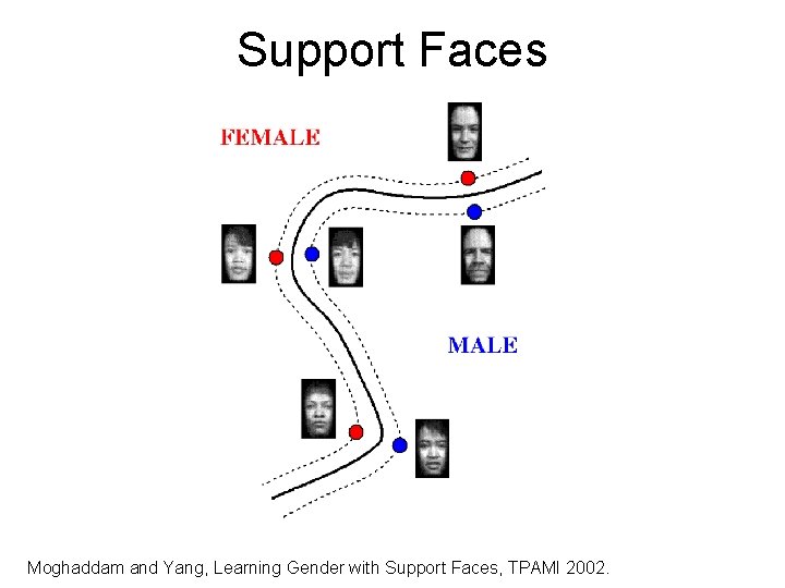
Example: learning gender with SVMs Moghaddam and Yang, Learning Gender with Support Faces, TPAMI 2002. Moghaddam and Yang, Face & Gesture 2000. Kristen Grauman

Learning gender with SVMs • Training examples: – 1044 males – 713 females • Experiment with various kernels, select Gaussian RBF Kristen Grauman

Support Faces Moghaddam and Yang, Learning Gender with Support Faces, TPAMI 2002.

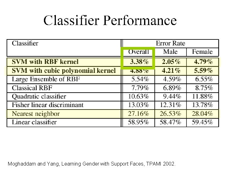
Moghaddam and Yang, Learning Gender with Support Faces, TPAMI 2002.

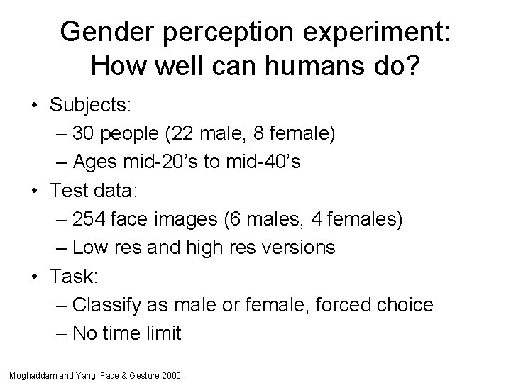
Gender perception experiment: How well can humans do? • Subjects: – 30 people (22 male, 8 female) – Ages mid-20’s to mid-40’s • Test data: – 254 face images (6 males, 4 females) – Low res and high res versions • Task: – Classify as male or female, forced choice – No time limit Moghaddam and Yang, Face & Gesture 2000.

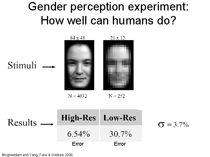
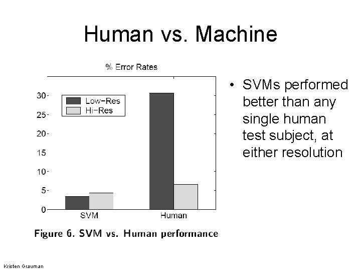
Gender perception experiment: How well can humans do? Error Moghaddam and Yang, Face & Gesture 2000. Error

Human vs. Machine • SVMs performed better than any single human test subject, at either resolution Kristen Grauman

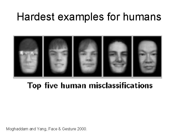
Hardest examples for humans Moghaddam and Yang, Face & Gesture 2000.

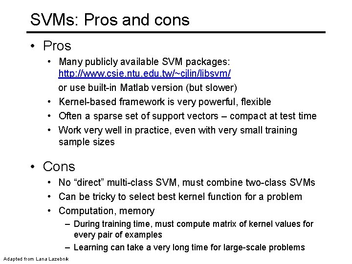
SVMs: Pros and cons • Pros • Many publicly available SVM packages: http: //www. csie. ntu. edu. tw/~cjlin/libsvm/ or use built-in Matlab version (but slower) • Kernel-based framework is very powerful, flexible • Often a sparse set of support vectors – compact at test time • Work very well in practice, even with very small training sample sizes • Cons • No “direct” multi-class SVM, must combine two-class SVMs • Can be tricky to select best kernel function for a problem • Computation, memory – During training time, must compute matrix of kernel values for every pair of examples – Learning can take a very long time for large-scale problems Adapted from Lana Lazebnik