CS 1699 Intro to Computer Vision Local Image

CS 1699: Intro to Computer Vision Local Image Features: Extraction and Description Prof. Adriana Kovashka University of Pittsburgh September 17, 2015

Announcement What: CS Welcome Party When: Friday, September 18, 2015 at 11: 00 AM Where: SENSQ 5317 Why (1): To learn about the CS Department, the CS Major and other interesting / useful things • Why (2): To meet other students and faculty • Why (3): To have some pizza! • •

Plan for today • Feature extraction / keypoint detection • Feature description • Homework due on Tuesday • Office hours today moved to 1 pm-2 pm tomorrow

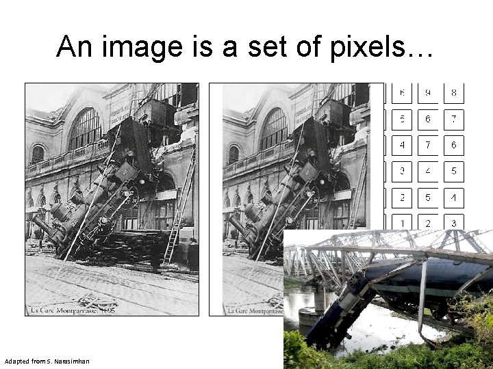
An image is a set of pixels… What we see Adapted from S. Narasimhan What a computer sees Source: S. Narasimhan

Problems with pixel representation • Not invariant to small changes – Translation – Illumination – etc. • Some parts of an image are more important than others • What do we want to represent?

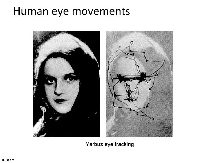
Interest points • Note: “interest points” = “keypoints”, also sometimes called “features” • Many applications – tracking: which points are good to track? – recognition: find patches likely to tell us something about object category – 3 D reconstruction: find correspondences across different views D. Hoiem

Human eye movements Yarbus eye tracking D. Hoiem

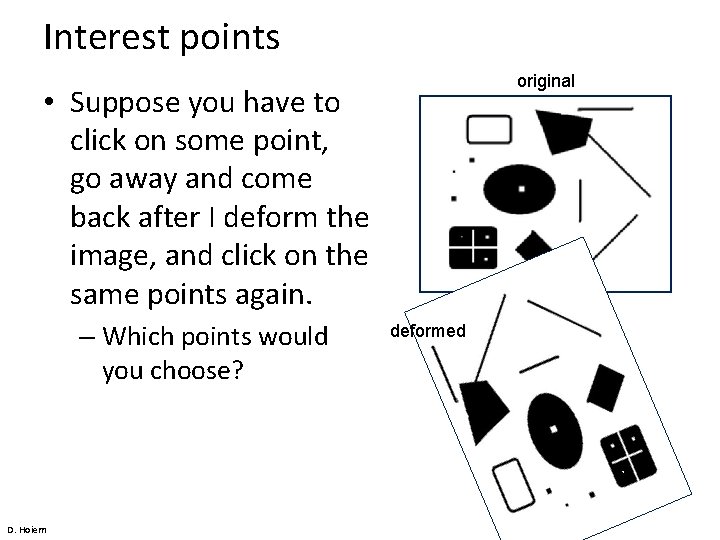
Interest points original • Suppose you have to click on some point, go away and come back after I deform the image, and click on the same points again. – Which points would you choose? D. Hoiem deformed

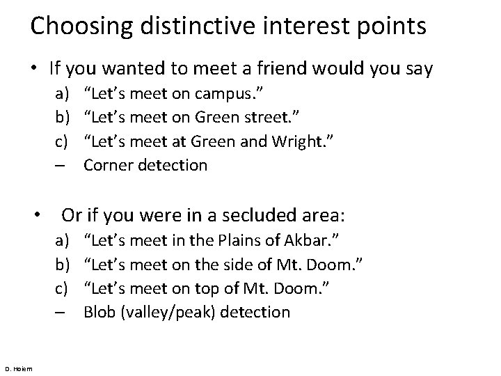
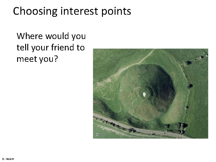
Choosing distinctive interest points • If you wanted to meet a friend would you say a) b) c) – “Let’s meet on campus. ” “Let’s meet on Green street. ” “Let’s meet at Green and Wright. ” Corner detection • Or if you were in a secluded area: a) b) c) – D. Hoiem “Let’s meet in the Plains of Akbar. ” “Let’s meet on the side of Mt. Doom. ” “Let’s meet on top of Mt. Doom. ” Blob (valley/peak) detection

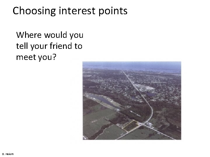
Choosing interest points Where would you tell your friend to meet you? D. Hoiem

Choosing interest points Where would you tell your friend to meet you? D. Hoiem

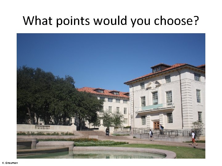
What points would you choose? K. Grauman

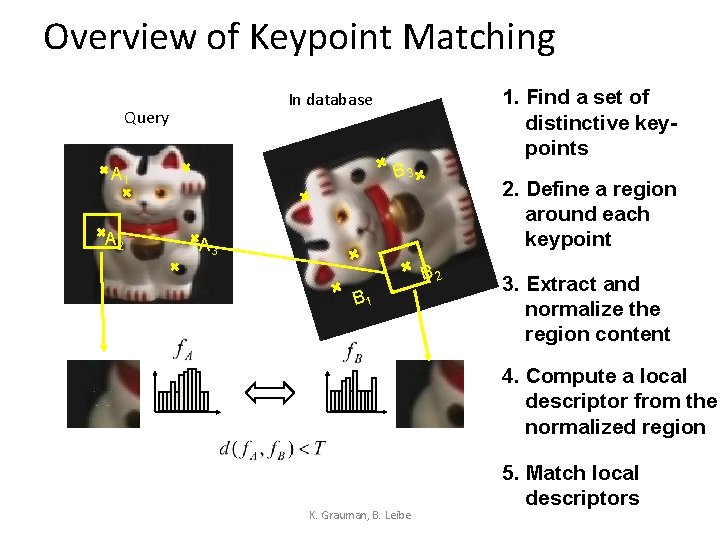
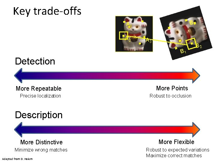
Overview of Keypoint Matching Query B 3 A 1 A 2 1. Find a set of distinctive keypoints In database 2. Define a region around each keypoint A 3 B 2 B 1 3. Extract and normalize the region content 4. Compute a local descriptor from the normalized region K. Grauman, B. Leibe 5. Match local descriptors

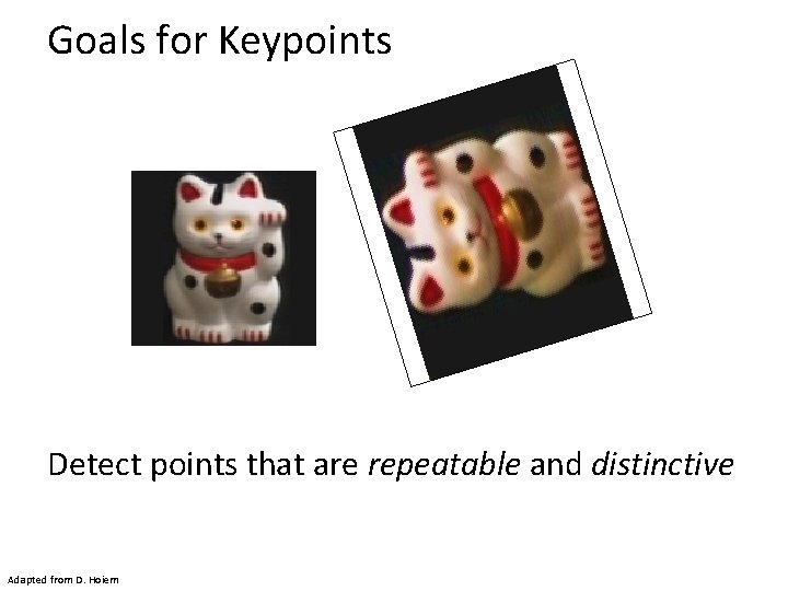
Goals for Keypoints Detect points that are repeatable and distinctive Adapted from D. Hoiem

Key trade-offs B 3 A 1 A 2 A 3 B 1 B 2 Detection More Repeatable Precise localization More Points Robust to occlusion Description More Distinctive More Flexible Minimize wrong matches Robust to expected variations Maximize correct matches Adapted from D. Hoiem

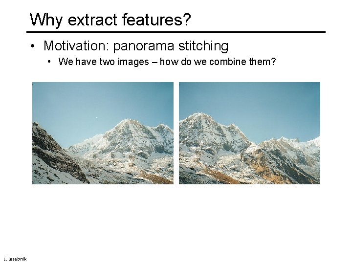
Why extract features? • Motivation: panorama stitching • We have two images – how do we combine them? L. Lazebnik

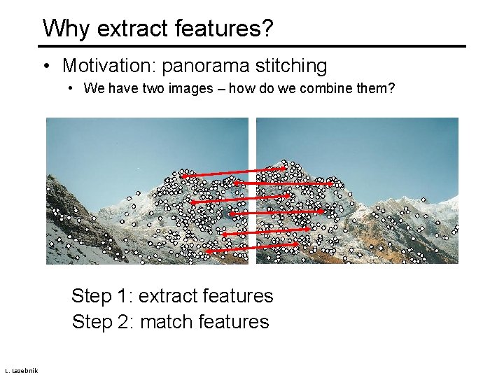
Why extract features? • Motivation: panorama stitching • We have two images – how do we combine them? Step 1: extract features Step 2: match features L. Lazebnik

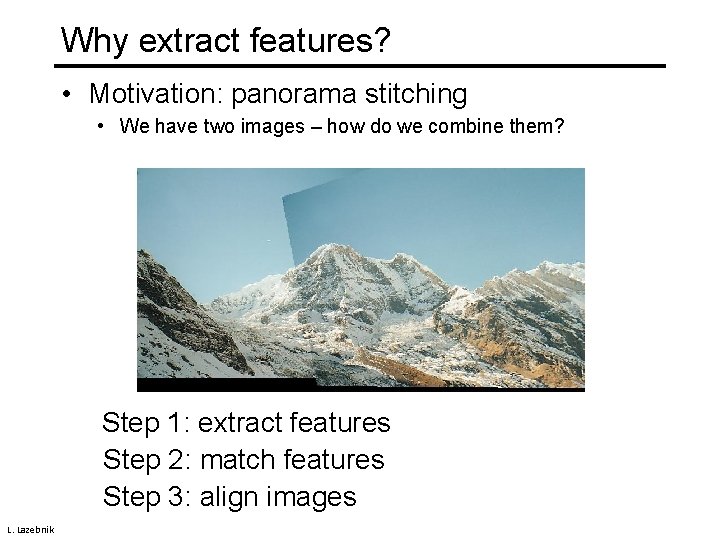
Why extract features? • Motivation: panorama stitching • We have two images – how do we combine them? Step 1: extract features Step 2: match features Step 3: align images L. Lazebnik

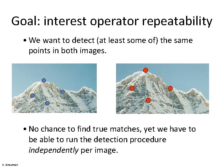
Goal: interest operator repeatability • We want to detect (at least some of) the same points in both images. • No chance to find true matches, yet we have to be able to run the detection procedure independently per image. K. Grauman

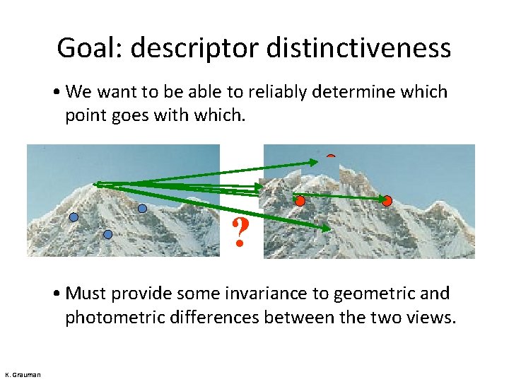
Goal: descriptor distinctiveness • We want to be able to reliably determine which point goes with which. ? • Must provide some invariance to geometric and photometric differences between the two views. K. Grauman

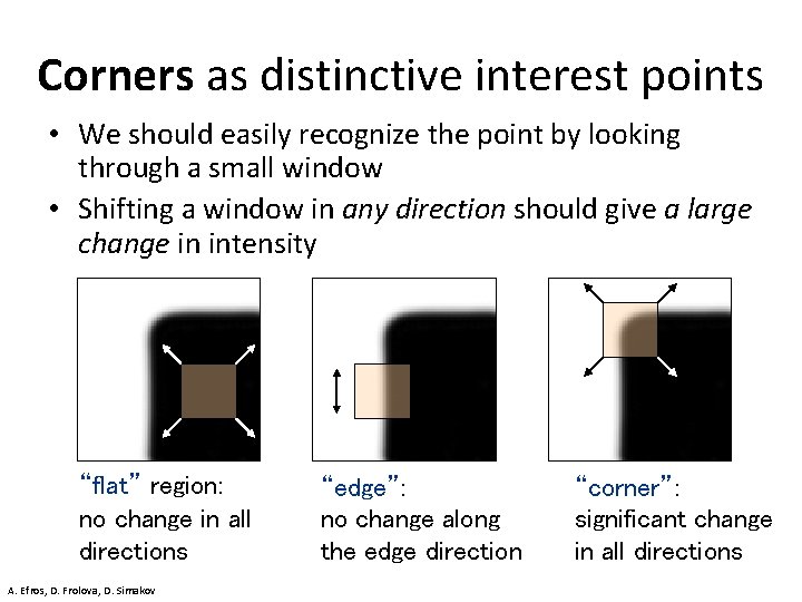
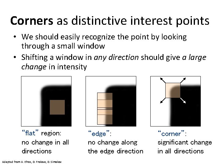
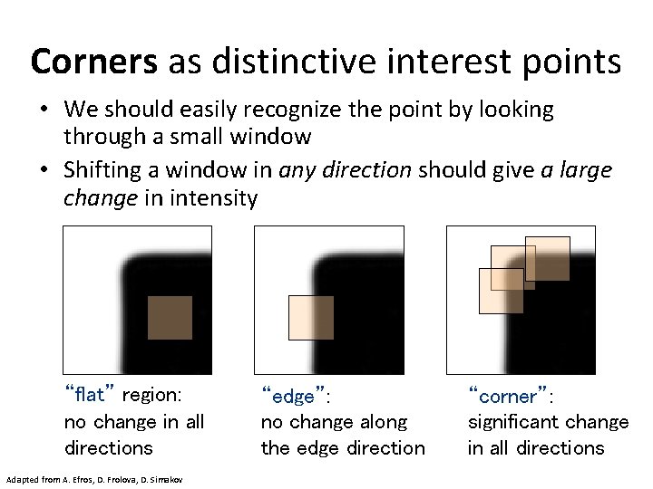
Corners as distinctive interest points • We should easily recognize the point by looking through a small window • Shifting a window in any direction should give a large change in intensity “flat” region: no change in all directions A. Efros, D. Frolova, D. Simakov “edge”: no change along the edge direction “corner”: significant change in all directions

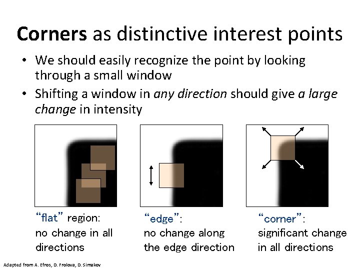
Corners as distinctive interest points • We should easily recognize the point by looking through a small window • Shifting a window in any direction should give a large change in intensity “flat” region: no change in all directions Adapted from A. Efros, D. Frolova, D. Simakov “edge”: no change along the edge direction “corner”: significant change in all directions

Corners as distinctive interest points • We should easily recognize the point by looking through a small window • Shifting a window in any direction should give a large change in intensity “flat” region: no change in all directions Adapted from A. Efros, D. Frolova, D. Simakov “edge”: no change along the edge direction “corner”: significant change in all directions

Corners as distinctive interest points • We should easily recognize the point by looking through a small window • Shifting a window in any direction should give a large change in intensity “flat” region: no change in all directions Adapted from A. Efros, D. Frolova, D. Simakov “edge”: no change along the edge direction “corner”: significant change in all directions

Corners as distinctive interest points • We should easily recognize the point by looking through a small window • Shifting a window in any direction should give a large change in intensity “flat” region: no change in all directions Adapted from A. Efros, D. Frolova, D. Simakov “edge”: no change along the edge direction “corner”: significant change in all directions

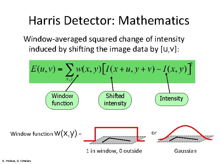
Harris Detector: Mathematics Window-averaged squared change of intensity induced by shifting the image data by [u, v]: Window function Shifted intensity Window function w(x, y) = or 1 in window, 0 outside D. Frolova, D. Simakov Intensity Gaussian

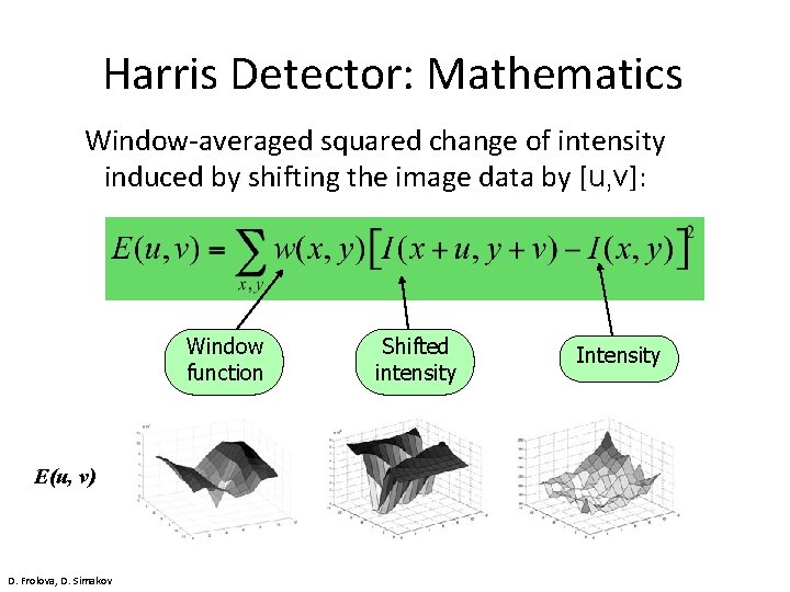
Harris Detector: Mathematics Window-averaged squared change of intensity induced by shifting the image data by [u, v]: Window function E(u, v) D. Frolova, D. Simakov Shifted intensity Intensity

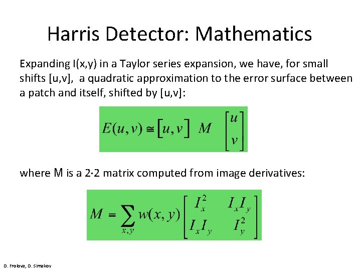
Harris Detector: Mathematics Expanding I(x, y) in a Taylor series expansion, we have, for small shifts [u, v], a quadratic approximation to the error surface between a patch and itself, shifted by [u, v]: where M is a 2× 2 matrix computed from image derivatives: D. Frolova, D. Simakov

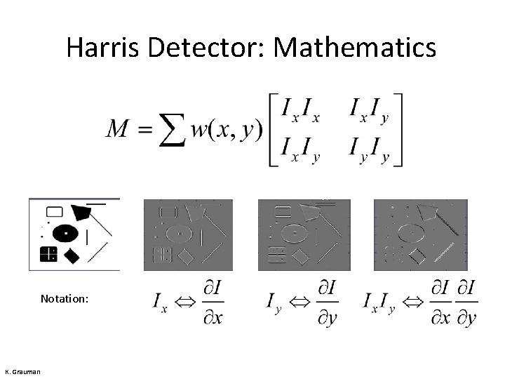
Harris Detector: Mathematics Notation: K. Grauman

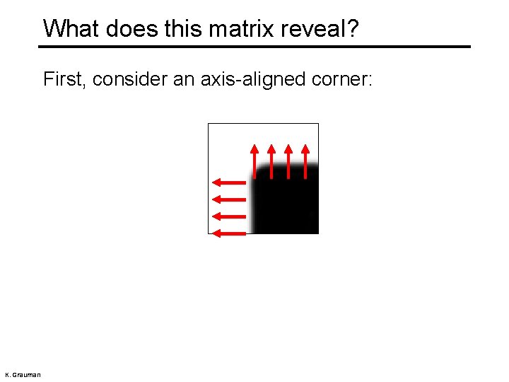
What does this matrix reveal? First, consider an axis-aligned corner: K. Grauman

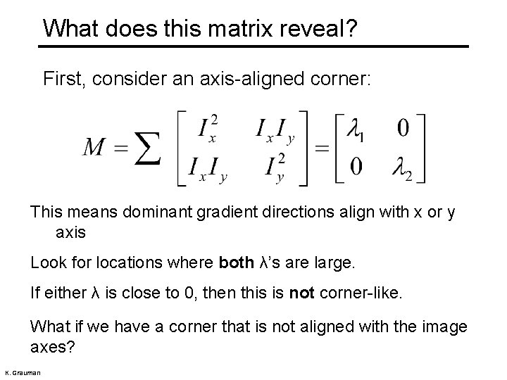
What does this matrix reveal? First, consider an axis-aligned corner: This means dominant gradient directions align with x or y axis Look for locations where both λ’s are large. If either λ is close to 0, then this is not corner-like. What if we have a corner that is not aligned with the image axes? K. Grauman

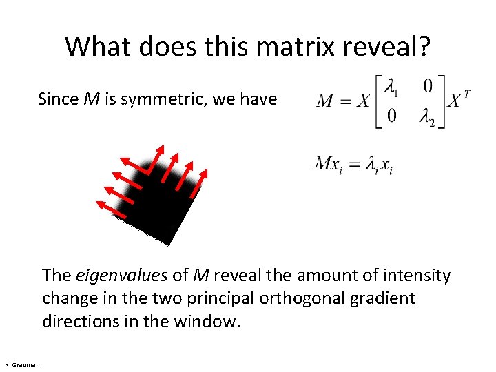
What does this matrix reveal? Since M is symmetric, we have The eigenvalues of M reveal the amount of intensity change in the two principal orthogonal gradient directions in the window. K. Grauman

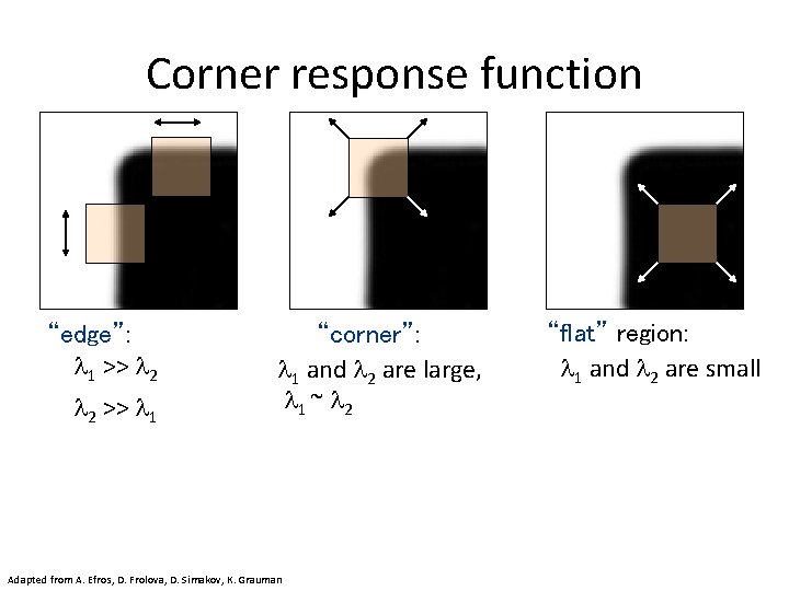
Corner response function “edge”: 1 >> 2 2 >> 1 “corner”: 1 and 2 are large, 1 ~ 2 Adapted from A. Efros, D. Frolova, D. Simakov, K. Grauman “flat” region: 1 and 2 are small

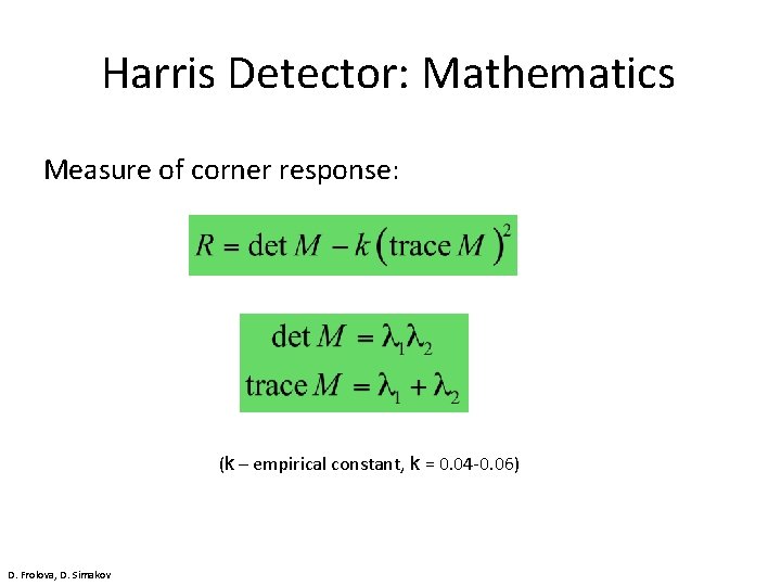
Harris Detector: Mathematics Measure of corner response: (k – empirical constant, k = 0. 04 -0. 06) D. Frolova, D. Simakov

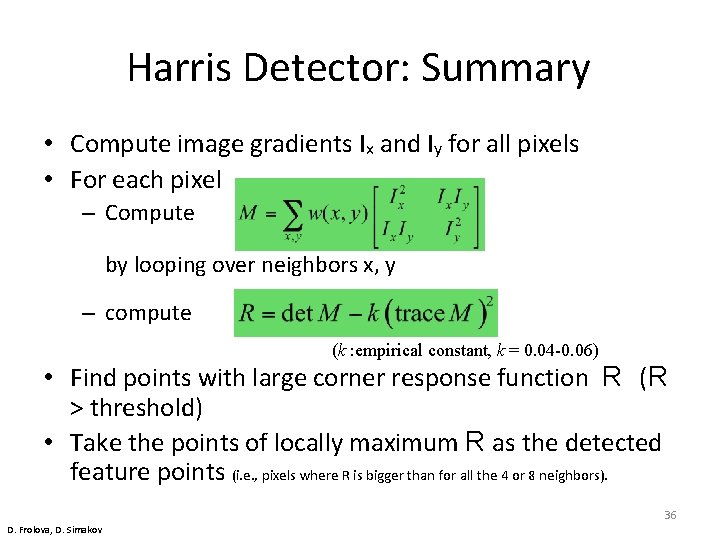
Harris Detector: Summary • Compute image gradients Ix and Iy for all pixels • For each pixel – Compute by looping over neighbors x, y – compute (k : empirical constant, k = 0. 04 -0. 06) • Find points with large corner response function R (R > threshold) • Take the points of locally maximum R as the detected feature points (i. e. , pixels where R is bigger than for all the 4 or 8 neighbors). 36 D. Frolova, D. Simakov

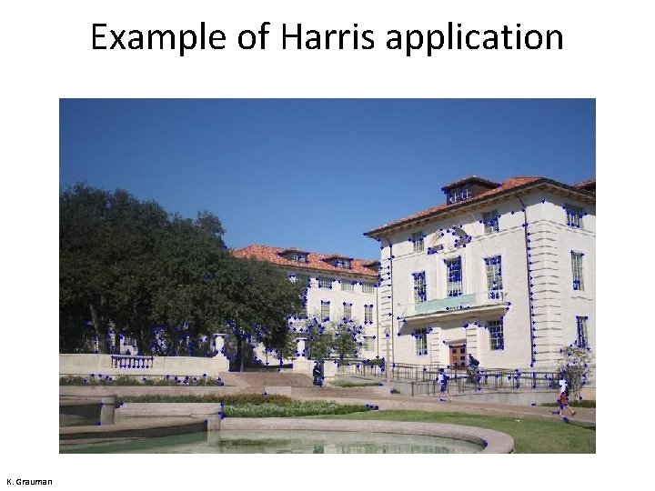
Example of Harris application K. Grauman

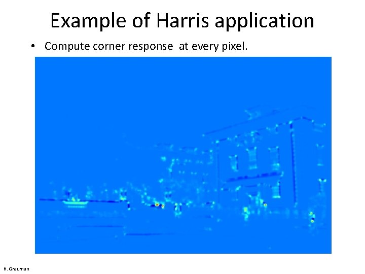
Example of Harris application • Compute corner response at every pixel. K. Grauman

Harris Detector – Responses [Harris 88] Effect: A very precise corner detector. D. Hoiem

Harris Detector - Responses [Harris 88] D. Hoiem

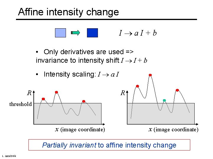
Affine intensity change I a. I+b • Only derivatives are used => invariance to intensity shift I I + b • Intensity scaling: I a I R R threshold x (image coordinate) Partially invariant to affine intensity change L. Lazebnik

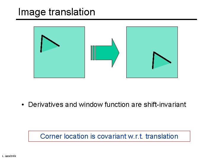
Image translation • Derivatives and window function are shift-invariant Corner location is covariant w. r. t. translation L. Lazebnik

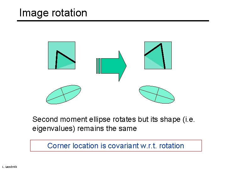
Image rotation Second moment ellipse rotates but its shape (i. e. eigenvalues) remains the same Corner location is covariant w. r. t. rotation L. Lazebnik

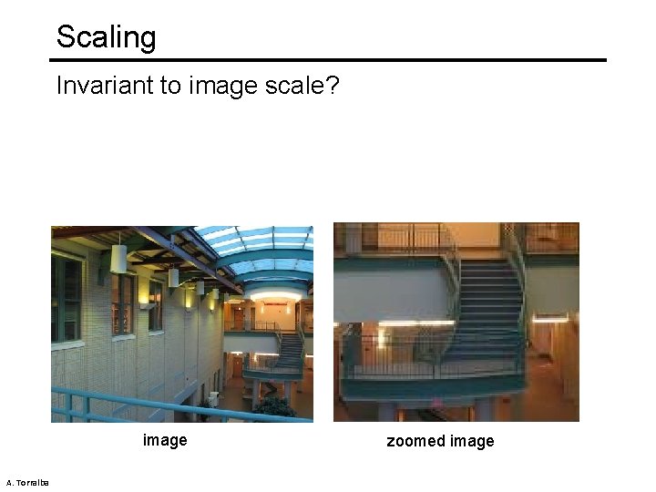
Scaling Invariant to image scale? image A. Torralba zoomed image

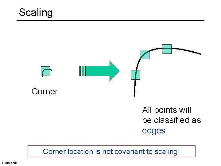
Scaling Corner All points will be classified as edges Corner location is not covariant to scaling! L. Lazebnik

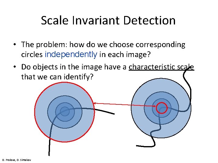
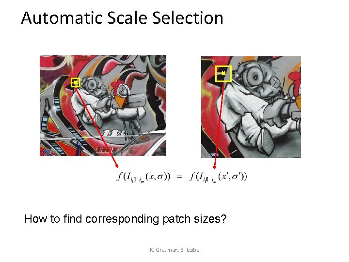
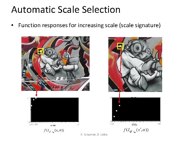
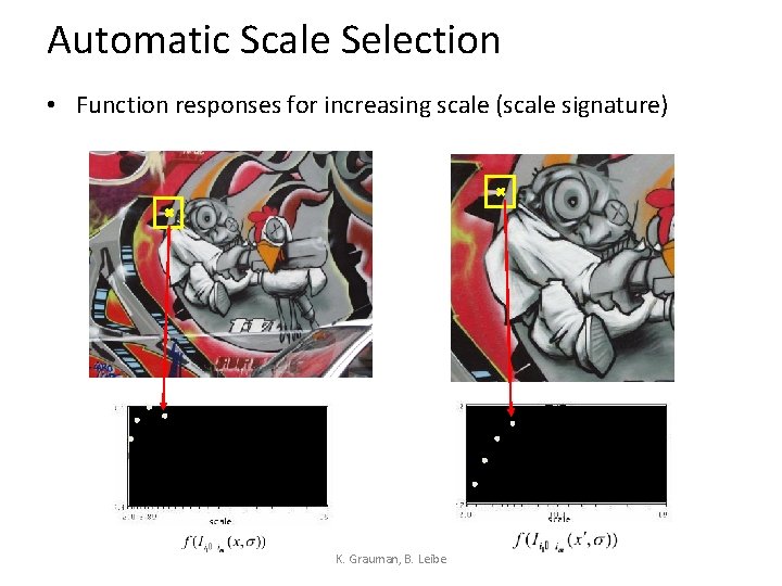
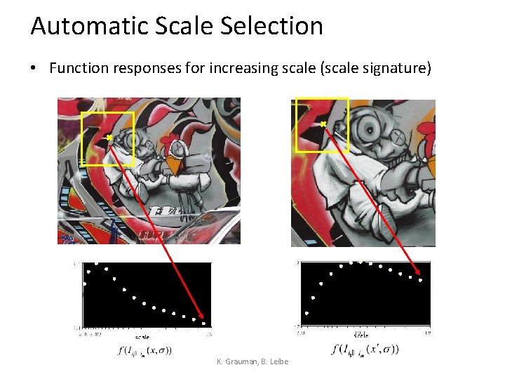
Scale Invariant Detection • The problem: how do we choose corresponding circles independently in each image? • Do objects in the image have a characteristic scale that we can identify? D. Frolova, D. Simakov

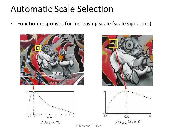
Automatic Scale Selection How to find corresponding patch sizes? K. Grauman, B. Leibe

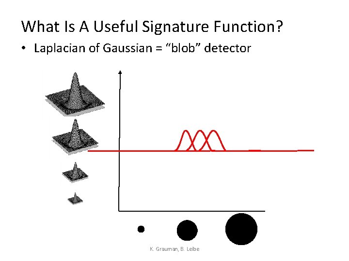
Automatic Scale Selection • Function responses for increasing scale (scale signature) K. Grauman, B. Leibe

Automatic Scale Selection • Function responses for increasing scale (scale signature) K. Grauman, B. Leibe

Automatic Scale Selection • Function responses for increasing scale (scale signature) K. Grauman, B. Leibe

Automatic Scale Selection • Function responses for increasing scale (scale signature) K. Grauman, B. Leibe

Automatic Scale Selection • Function responses for increasing scale (scale signature) K. Grauman, B. Leibe

Automatic Scale Selection • Function responses for increasing scale (scale signature) K. Grauman, B. Leibe

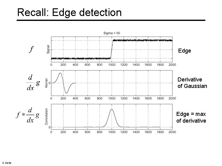
Recall: Edge detection f Edge Derivative of Gaussian Edge = max of derivative S. Seitz

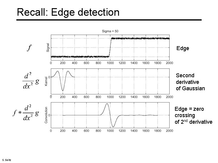
Recall: Edge detection f Edge Second derivative of Gaussian Edge = zero crossing of 2 nd derivative S. Seitz

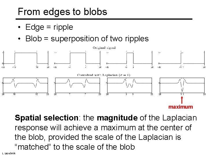
From edges to blobs • Edge = ripple • Blob = superposition of two ripples maximum Spatial selection: the magnitude of the Laplacian response will achieve a maximum at the center of the blob, provided the scale of the Laplacian is “matched” to the scale of the blob L. Lazebnik

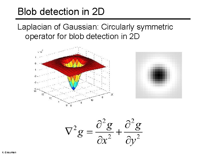
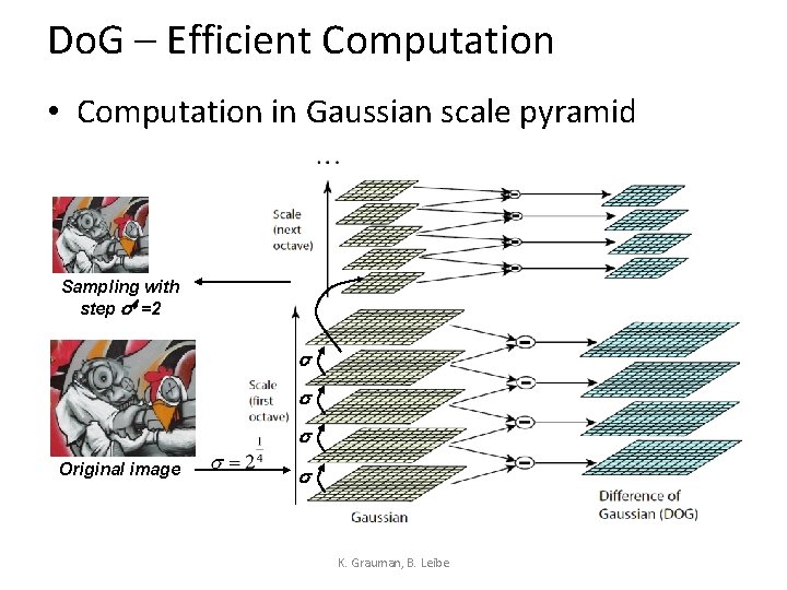
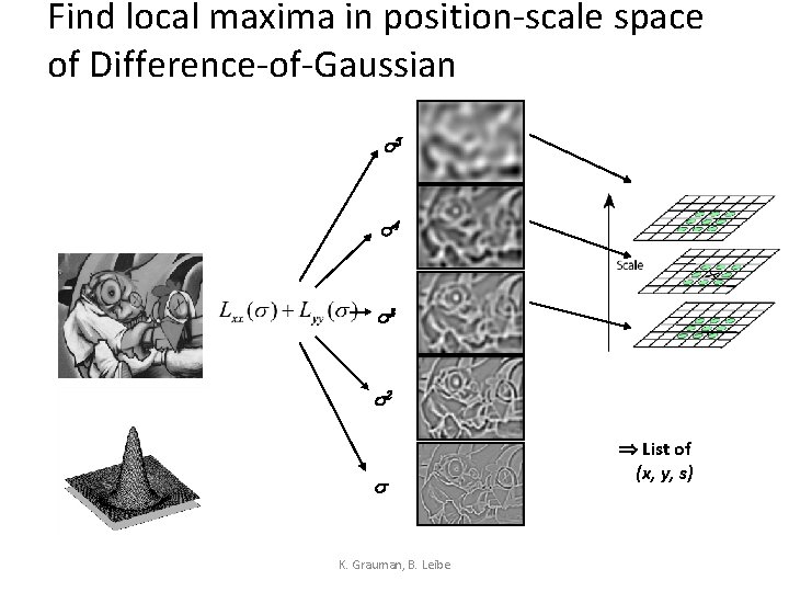
Blob detection in 2 D Laplacian of Gaussian: Circularly symmetric operator for blob detection in 2 D K. Grauman

What Is A Useful Signature Function? • Laplacian of Gaussian = “blob” detector K. Grauman, B. Leibe

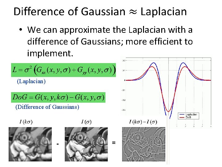
• We can approximate the Laplacian with a difference of Gaussians; more efficient to implement. (Laplacian) (Difference of Gaussians)

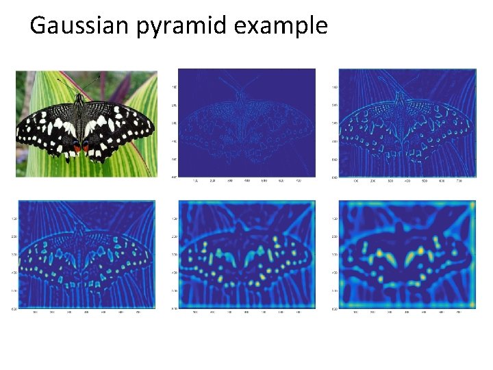
Gaussian pyramid example

Do. G – Efficient Computation • Computation in Gaussian scale pyramid Sampling with step s 4 =2 s s s Original image s K. Grauman, B. Leibe

Find local maxima in position-scale space of Difference-of-Gaussian s 5 s 4 s 3 s 2 s K. Grauman, B. Leibe List of (x, y, s)

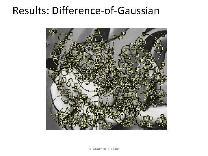
Results: Difference-of-Gaussian K. Grauman, B. Leibe

Gaussian pyramid example

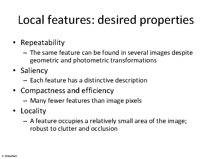
Local features: desired properties • Repeatability – The same feature can be found in several images despite geometric and photometric transformations • Saliency – Each feature has a distinctive description • Compactness and efficiency – Many fewer features than image pixels • Locality – A feature occupies a relatively small area of the image; robust to clutter and occlusion K. Grauman

Plan for today • Feature extraction / keypoint detection – Corners – Blobs • Feature description

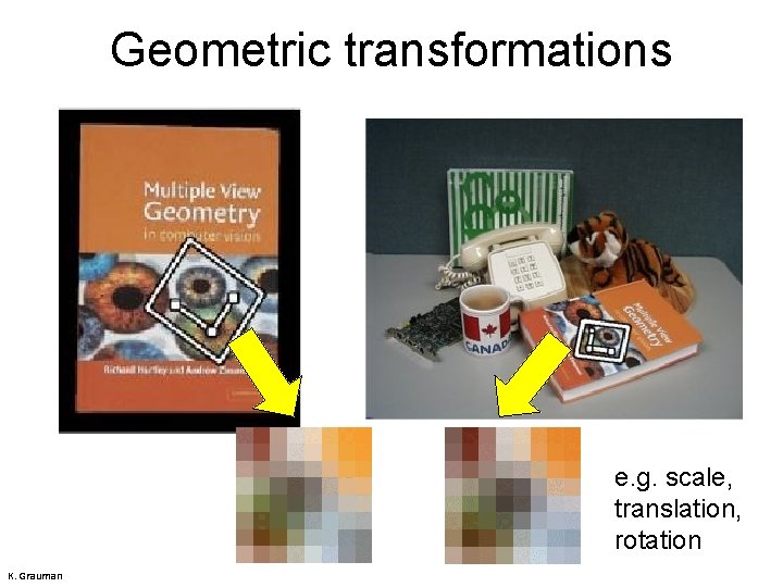
Geometric transformations e. g. scale, translation, rotation K. Grauman

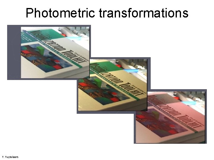
Photometric transformations T. Tuytelaars

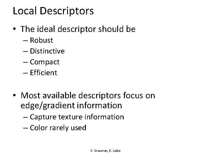
Local Descriptors • The ideal descriptor should be – Robust – Distinctive – Compact – Efficient • Most available descriptors focus on edge/gradient information – Capture texture information – Color rarely used K. Grauman, B. Leibe

Local Descriptors: SIFT Descriptor [Lowe, ICCV 1999] Histogram of oriented gradients • Captures important texture information • Robust to small translations / affine deformations K. Grauman, B. Leibe

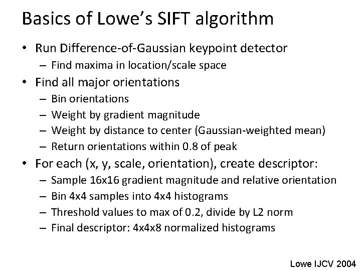
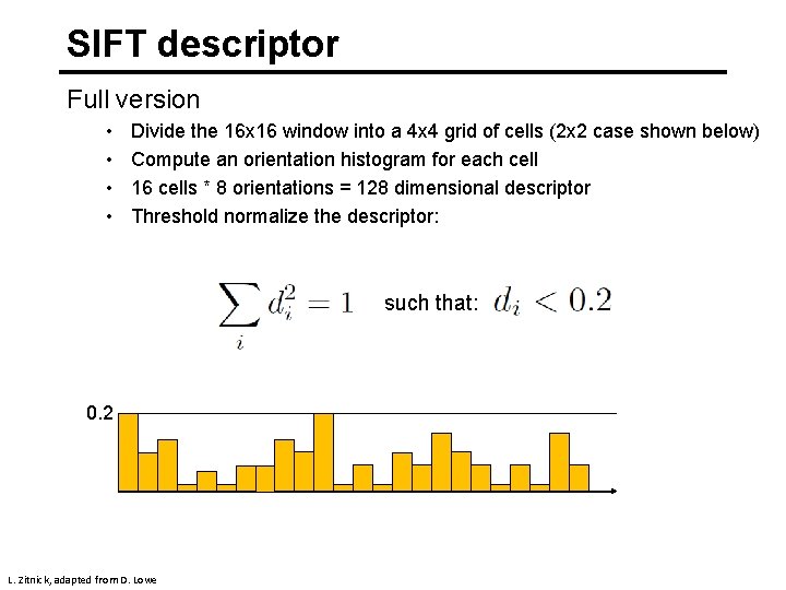
Basics of Lowe’s SIFT algorithm • Run Difference-of-Gaussian keypoint detector – Find maxima in location/scale space • Find all major orientations – – Bin orientations Weight by gradient magnitude Weight by distance to center (Gaussian-weighted mean) Return orientations within 0. 8 of peak • For each (x, y, scale, orientation), create descriptor: – – Sample 16 x 16 gradient magnitude and relative orientation Bin 4 x 4 samples into 4 x 4 histograms Threshold values to max of 0. 2, divide by L 2 norm Final descriptor: 4 x 4 x 8 normalized histograms Lowe IJCV 2004

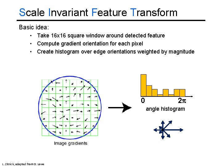
Scale Invariant Feature Transform Basic idea: • Take 16 x 16 square window around detected feature • Compute gradient orientation for each pixel • Create histogram over edge orientations weighted by magnitude 0 2 angle histogram L. Zitnick, adapted from D. Lowe

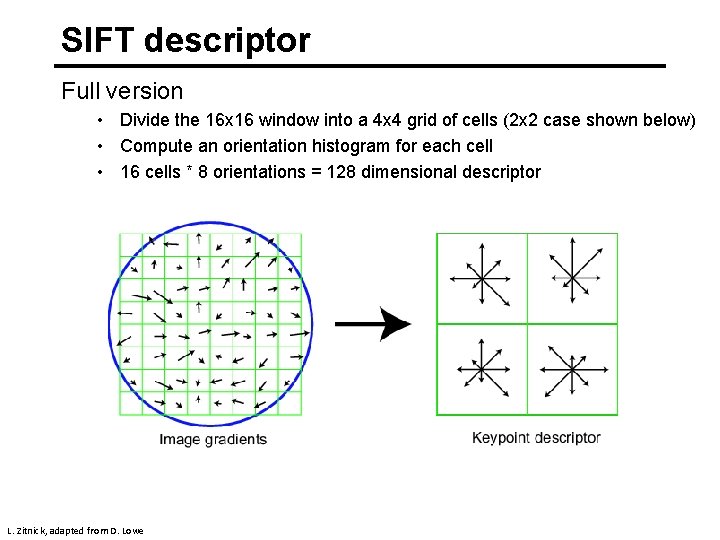
SIFT descriptor Full version • Divide the 16 x 16 window into a 4 x 4 grid of cells (2 x 2 case shown below) • Compute an orientation histogram for each cell • 16 cells * 8 orientations = 128 dimensional descriptor L. Zitnick, adapted from D. Lowe

SIFT descriptor Full version • • Divide the 16 x 16 window into a 4 x 4 grid of cells (2 x 2 case shown below) Compute an orientation histogram for each cell 16 cells * 8 orientations = 128 dimensional descriptor Threshold normalize the descriptor: such that: 0. 2 L. Zitnick, adapted from D. Lowe

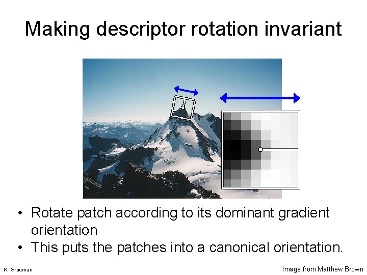
Making descriptor rotation invariant CSE 576: Computer Vision • Rotate patch according to its dominant gradient orientation • This puts the patches into a canonical orientation. K. Grauman Image from Matthew Brown

SIFT descriptor [Lowe 2004] • Extraordinarily robust matching technique • Can handle changes in viewpoint • Up to about 60 degree out of plane rotation • Can handle significant changes in illumination • Sometimes even day vs. night (below) • • Fast and efficient—can run in real time Lots of code available • S. Seitz http: //people. csail. mit. edu/albert/ladypack/wiki/index. php/Known_implementations_of_SIFT

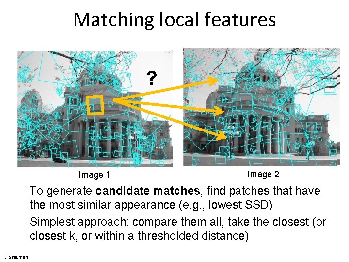
Matching local features ? Image 1 Image 2 To generate candidate matches, find patches that have the most similar appearance (e. g. , lowest SSD) Simplest approach: compare them all, take the closest (or closest k, or within a thresholded distance) K. Grauman

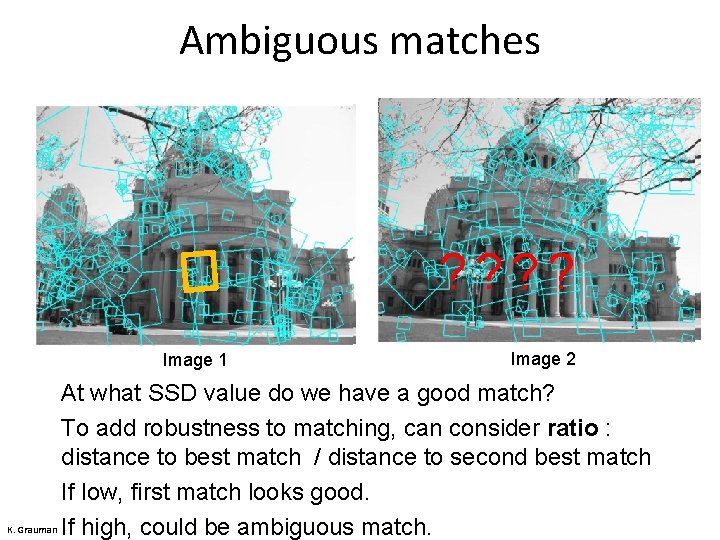
Ambiguous matches ? ? Image 1 Image 2 At what SSD value do we have a good match? To add robustness to matching, can consider ratio : distance to best match / distance to second best match If low, first match looks good. K. Grauman If high, could be ambiguous match.

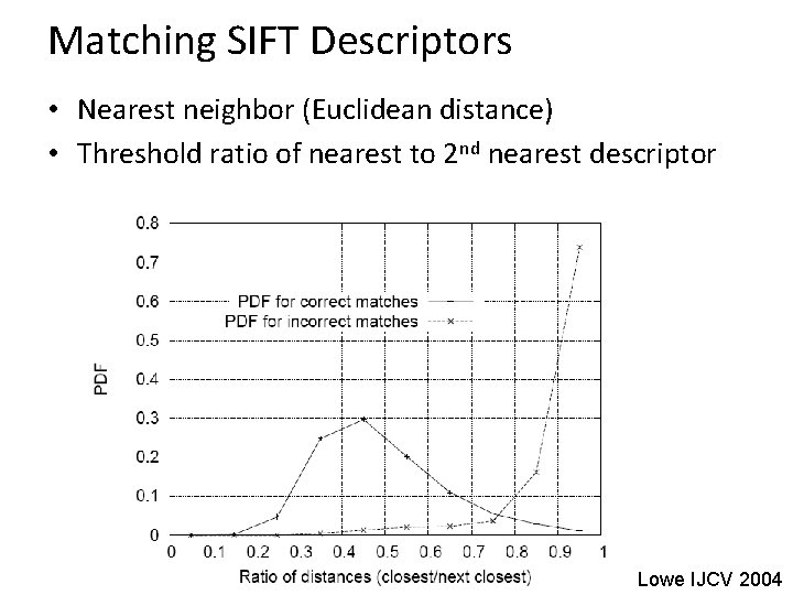
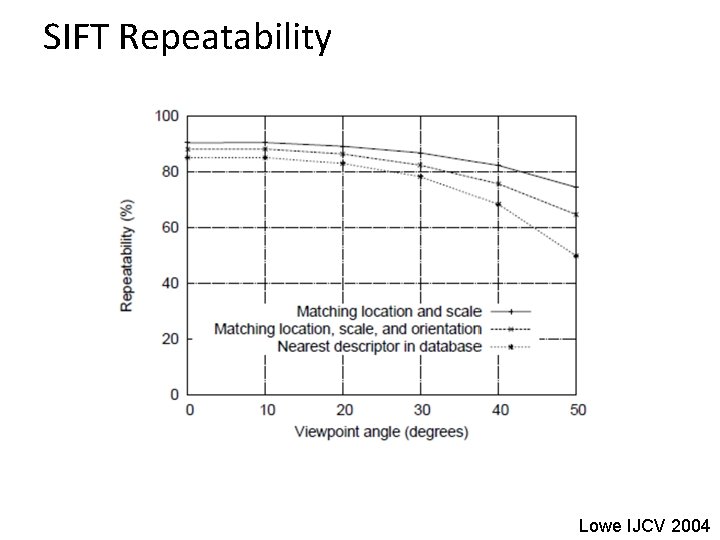
Matching SIFT Descriptors • Nearest neighbor (Euclidean distance) • Threshold ratio of nearest to 2 nd nearest descriptor Lowe IJCV 2004

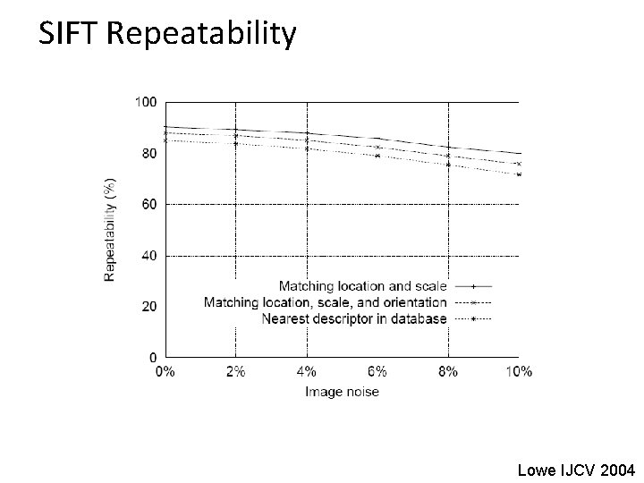
SIFT Repeatability Lowe IJCV 2004

SIFT Repeatability Lowe IJCV 2004

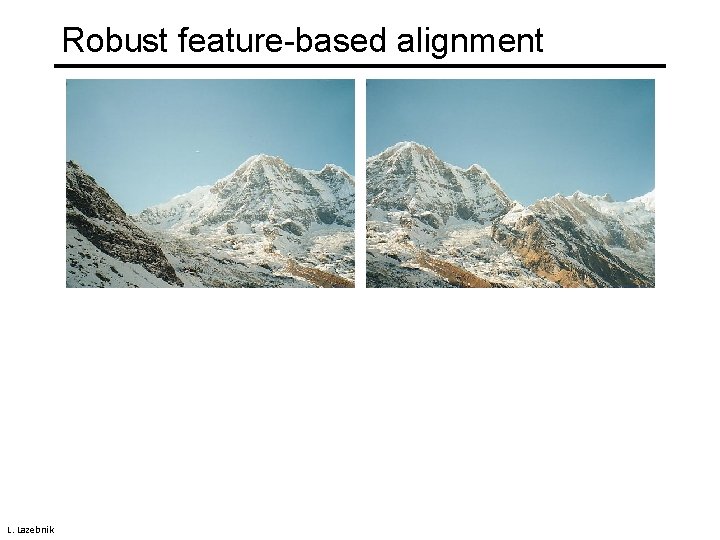
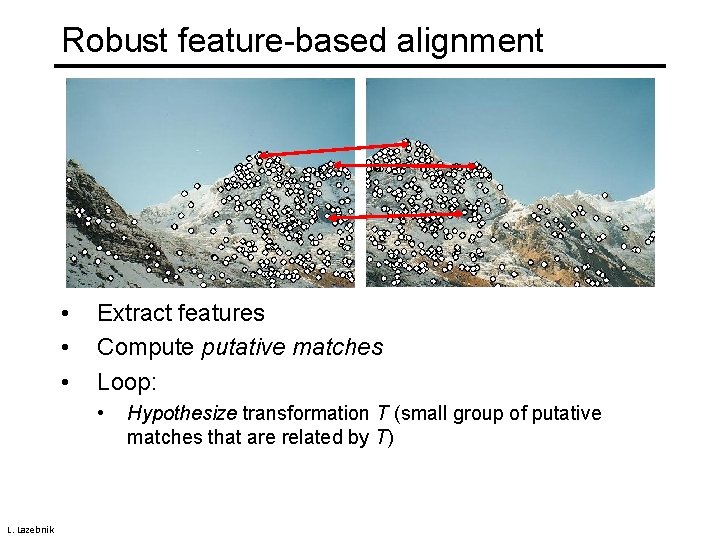
Robust feature-based alignment L. Lazebnik

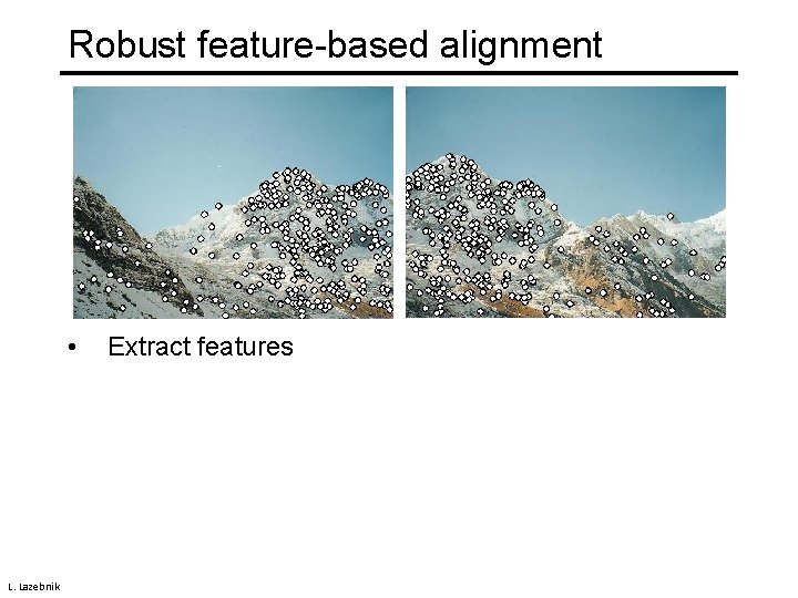
Robust feature-based alignment • L. Lazebnik Extract features

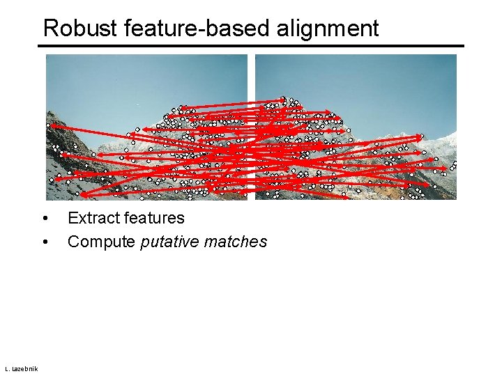
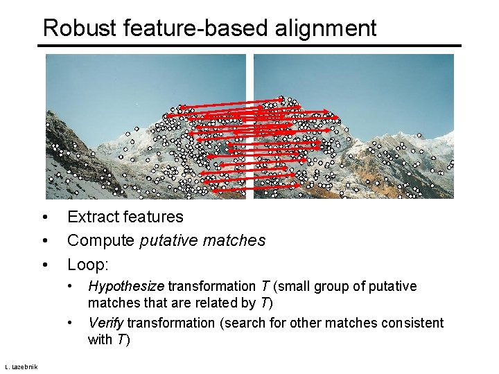
Robust feature-based alignment • • L. Lazebnik Extract features Compute putative matches

Robust feature-based alignment • • • Extract features Compute putative matches Loop: • L. Lazebnik Hypothesize transformation T (small group of putative matches that are related by T)

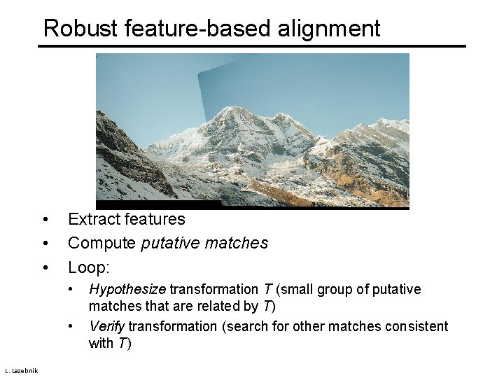
Robust feature-based alignment • • • Extract features Compute putative matches Loop: • • L. Lazebnik Hypothesize transformation T (small group of putative matches that are related by T) Verify transformation (search for other matches consistent with T)

Robust feature-based alignment • • • Extract features Compute putative matches Loop: • • L. Lazebnik Hypothesize transformation T (small group of putative matches that are related by T) Verify transformation (search for other matches consistent with T)

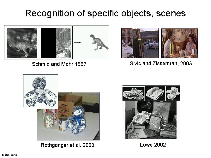
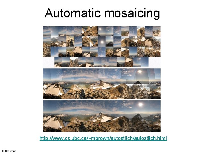
Applications of local invariant features • • • Image alignment Indexing and retrieval Recognition Robot navigation 3 D reconstruction Wide baseline stereo Panoramas Motion tracking … Adapted from K. Grauman and L. Lazebnik

Recognition of specific objects, scenes Schmid and Mohr 1997 Rothganger et al. 2003 K. Grauman Sivic and Zisserman, 2003 Lowe 2002

Wide baseline stereo [Image from T. Tuytelaars ECCV 2006 tutorial]

Automatic mosaicing http: //www. cs. ubc. ca/~mbrown/autostitch. html K. Grauman

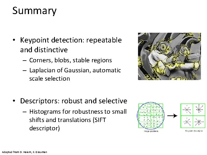
Summary • Keypoint detection: repeatable and distinctive – Corners, blobs, stable regions – Laplacian of Gaussian, automatic scale selection • Descriptors: robust and selective – Histograms for robustness to small shifts and translations (SIFT descriptor) Adapted from D. Hoiem, K. Grauman