CS 1674 Intro to Computer Vision Filtering and

CS 1674: Intro to Computer Vision Filtering and Texture Prof. Adriana Kovashka University of Pittsburgh September 12, 2016

Reminder • HW 1 P, HW 2 W due tonight, 11: 59 pm

Plan for today • Filters: math and properties • Types of filters – Linear • Smoothing • Other – Non-linear • Median • Texture representation with filters

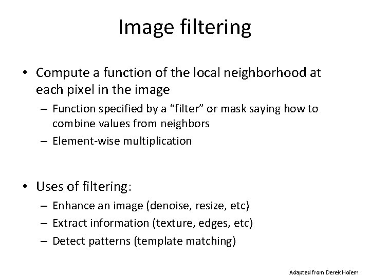
Image filtering • Compute a function of the local neighborhood at each pixel in the image – Function specified by a “filter” or mask saying how to combine values from neighbors – Element-wise multiplication • Uses of filtering: – Enhance an image (denoise, resize, etc) – Extract information (texture, edges, etc) – Detect patterns (template matching) Adapted from Derek Hoiem

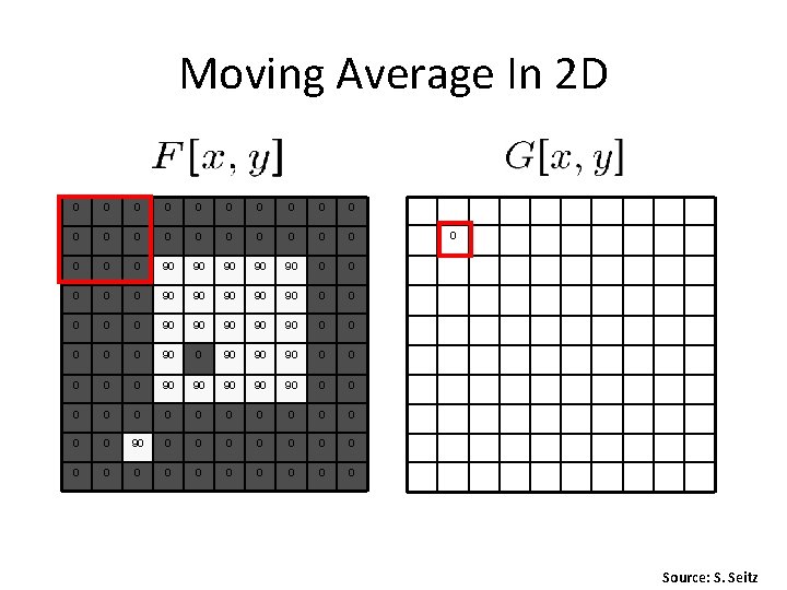
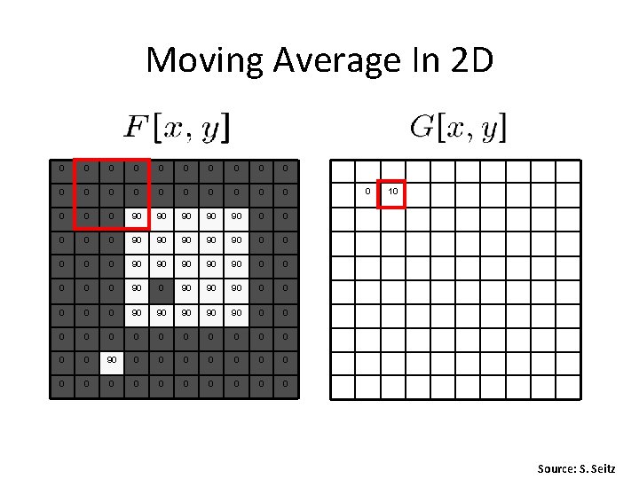
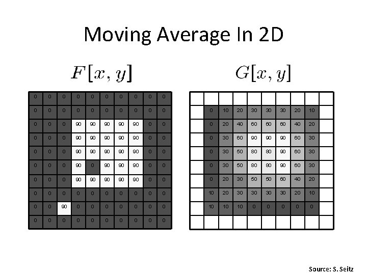
Moving Average In 2 D 0 0 0 0 0 0 90 90 90 0 0 90 90 90 0 90 90 90 0 0 0 0 0 0 0 0 0 Source: S. Seitz

Moving Average In 2 D 0 0 0 0 0 0 90 90 90 0 0 90 90 90 0 90 90 90 0 0 0 0 0 0 0 0 0 10 Source: S. Seitz

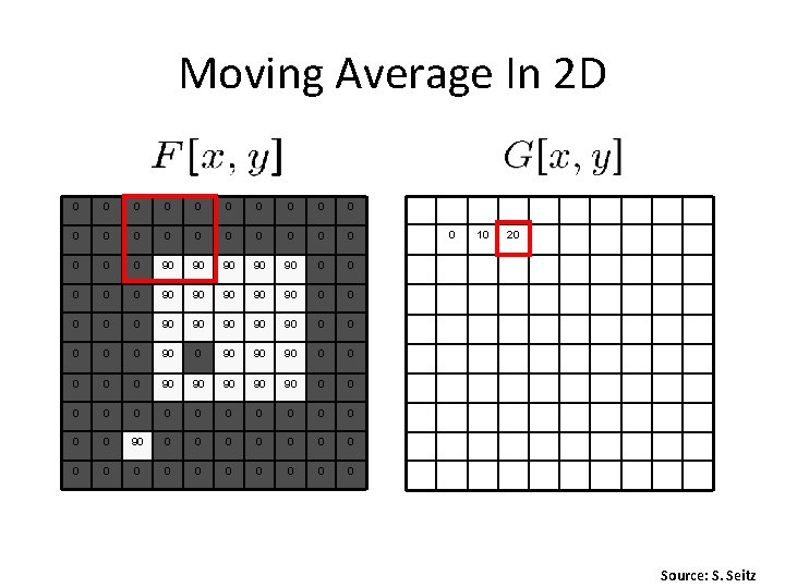
Moving Average In 2 D 0 0 0 0 0 0 90 90 90 0 0 90 90 90 0 90 90 90 0 0 0 0 0 0 0 0 0 10 20 Source: S. Seitz

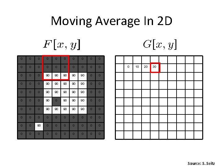
Moving Average In 2 D 0 0 0 0 0 0 90 90 90 0 0 90 90 90 0 90 90 90 0 0 0 0 0 0 0 0 0 10 20 30 Source: S. Seitz

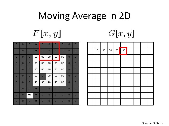
Moving Average In 2 D 0 0 0 0 0 0 90 90 90 0 0 90 90 90 0 90 90 90 0 0 0 0 0 0 0 0 0 10 20 30 30 Source: S. Seitz

Moving Average In 2 D 0 0 0 0 0 0 10 20 30 30 30 20 10 0 90 90 90 0 20 40 60 60 60 40 20 0 90 90 90 0 30 60 90 90 90 60 30 0 90 90 90 0 30 50 80 80 90 60 30 0 90 90 90 0 20 30 50 50 60 40 20 0 0 10 20 30 30 20 10 0 0 90 0 0 0 10 10 10 0 0 0 Source: S. Seitz

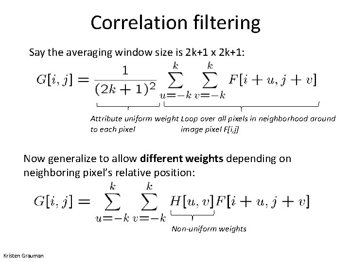
Correlation filtering Say the averaging window size is 2 k+1 x 2 k+1: Attribute uniform weight Loop over all pixels in neighborhood around to each pixel image pixel F[i, j] Now generalize to allow different weights depending on neighboring pixel’s relative position: Non-uniform weights Kristen Grauman

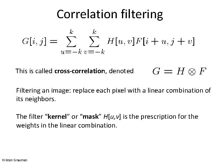
Correlation filtering This is called cross-correlation, denoted Filtering an image: replace each pixel with a linear combination of its neighbors. The filter “kernel” or “mask” H[u, v] is the prescription for the weights in the linear combination. Kristen Grauman

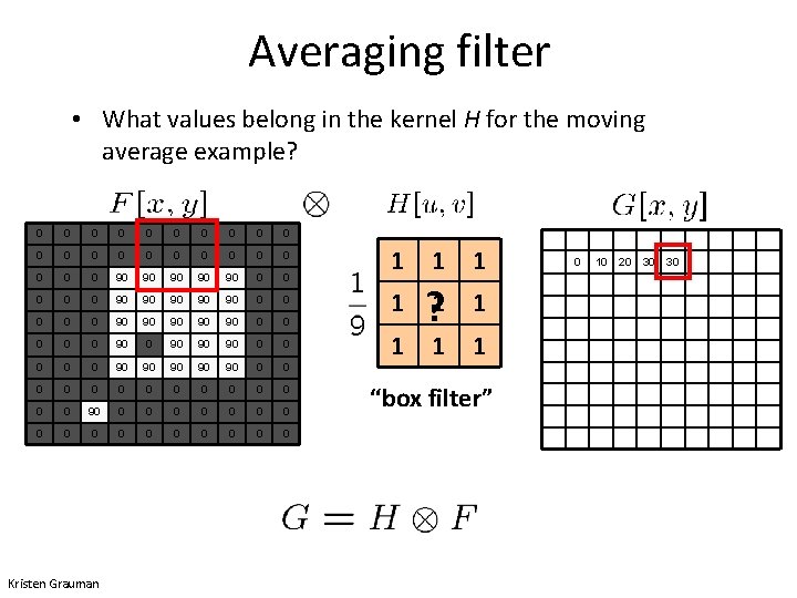
Averaging filter • What values belong in the kernel H for the moving average example? 0 0 0 0 0 0 90 90 90 0 0 90 90 90 0 90 90 90 0 0 0 0 0 0 0 0 0 0 Kristen Grauman 1 1 ? 1 1 1 “box filter” 0 10 20 30 30

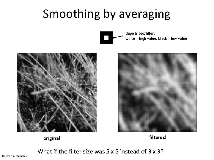
Smoothing by averaging depicts box filter: white = high value, black = low value original Kristen Grauman filtered What if the filter size was 5 x 5 instead of 3 x 3?

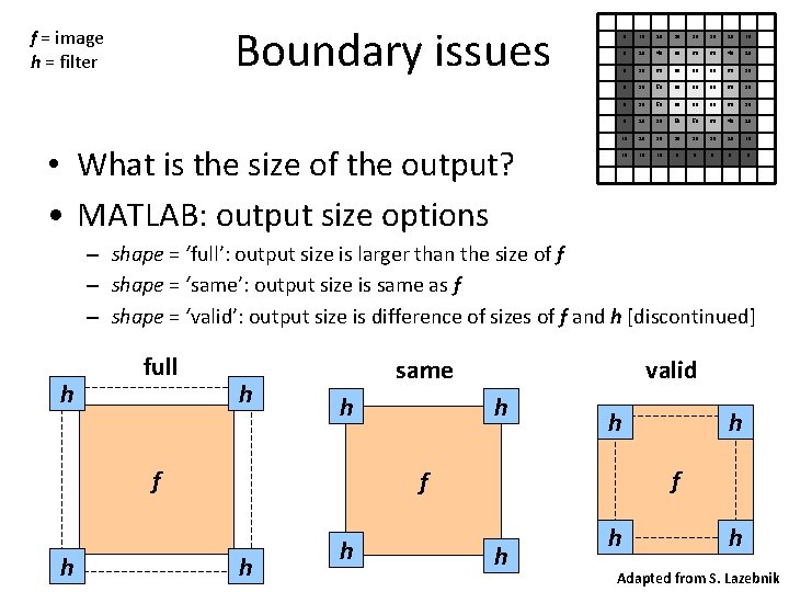
Boundary issues f = image h = filter • What is the size of the output? • MATLAB: output size options 0 10 20 30 30 30 20 10 0 20 40 60 60 60 40 20 0 30 60 90 90 90 60 30 50 80 80 90 60 30 0 20 30 50 50 60 40 20 10 20 30 30 20 10 10 0 0 – shape = ‘full’: output size is larger than the size of f – shape = ‘same’: output size is same as f – shape = ‘valid’: output size is difference of sizes of f and h [discontinued] h full h same h f h valid h h f f h h h Adapted from S. Lazebnik

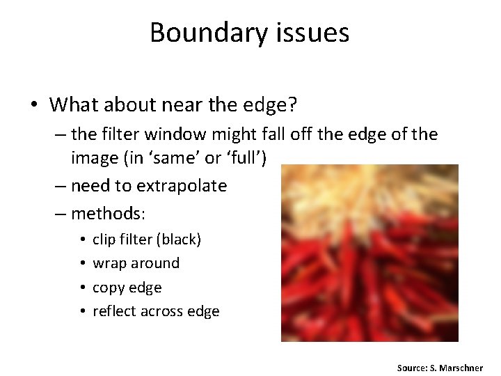
Boundary issues • What about near the edge? – the filter window might fall off the edge of the image (in ‘same’ or ‘full’) – need to extrapolate – methods: • • clip filter (black) wrap around copy edge reflect across edge Source: S. Marschner

Boundary issues • What about near the edge? – the filter window might fall off the edge of the image (in ‘same’ or ‘full’) – need to extrapolate – methods (MATLAB): • • clip filter (black): wrap around: copy edge: reflect across edge: imfilter(f, g, 0) imfilter(f, g, ‘circular’) imfilter(f, g, ‘replicate’) imfilter(f, g, ‘symmetric’) Source: S. Marschner

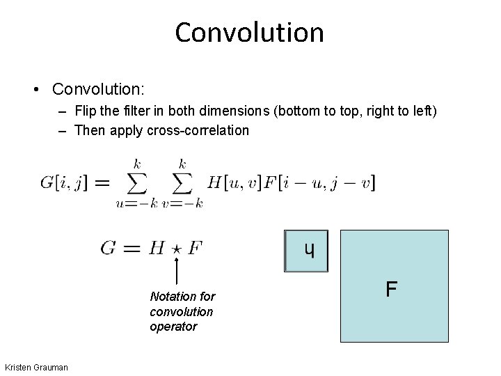
Convolution • Convolution: – Flip the filter in both dimensions (bottom to top, right to left) – Then apply cross-correlation h Notation for convolution operator Kristen Grauman F

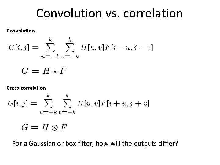
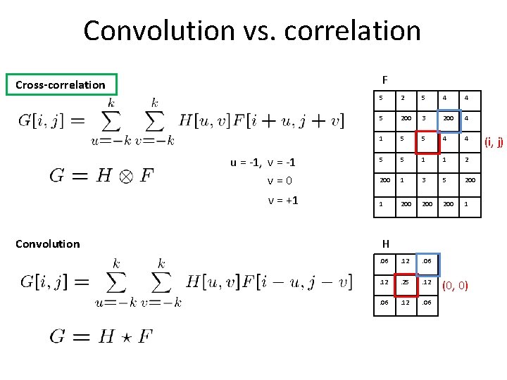
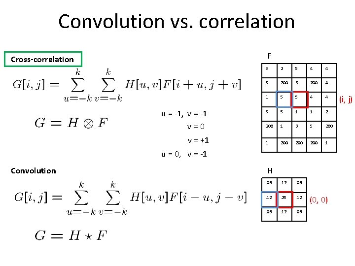
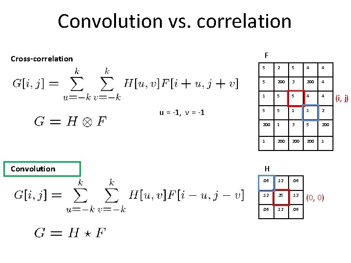
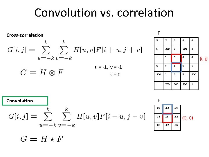
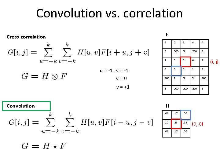
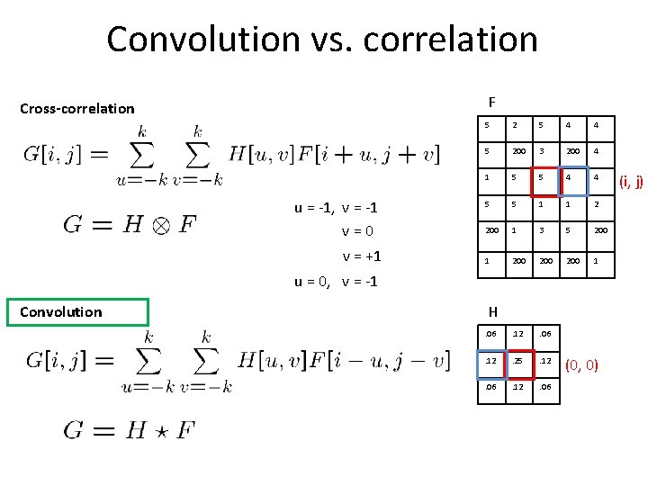
Convolution vs. correlation Convolution Cross-correlation For a Gaussian or box filter, how will the outputs differ?

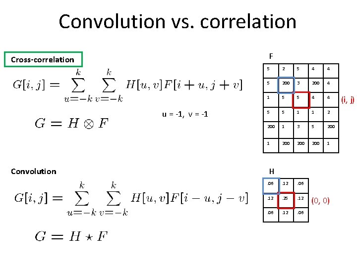
Convolution vs. correlation F Cross-correlation u = -1, v = -1 Convolution 5 2 5 4 4 5 200 3 200 4 1 5 5 4 4 5 5 1 1 2 200 1 3 5 200 1 200 200 1 . 06 . 12 . 25 . 12 . 06 H (0, 0) (i, j)

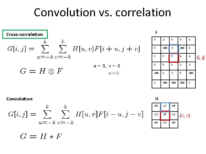
Convolution vs. correlation F Cross-correlation u = -1, v = -1 v=0 Convolution 5 2 5 4 4 5 200 3 200 4 1 5 5 4 4 5 5 1 1 2 200 1 3 5 200 1 200 200 1 . 06 . 12 . 25 . 12 . 06 H (0, 0) (i, j)

Convolution vs. correlation F Cross-correlation u = -1, v = -1 v=0 v = +1 Convolution 5 2 5 4 4 5 200 3 200 4 1 5 5 4 4 5 5 1 1 2 200 1 3 5 200 1 200 200 1 . 06 . 12 . 25 . 12 . 06 H (0, 0) (i, j)

Convolution vs. correlation F Cross-correlation u = -1, v = -1 v=0 v = +1 5 2 5 4 4 5 200 3 200 4 1 5 5 4 4 5 5 1 1 2 200 1 3 5 200 1 200 200 1 . 06 . 12 . 25 . 12 . 06 u = 0, v = -1 Convolution H (0, 0) (i, j)

Convolution vs. correlation F Cross-correlation u = -1, v = -1 Convolution 5 2 5 4 4 5 200 3 200 4 1 5 5 4 4 5 5 1 1 2 200 1 3 5 200 1 200 200 1 . 06 . 12 . 25 . 12 . 06 H (0, 0) (i, j)

Convolution vs. correlation F Cross-correlation u = -1, v = -1 v=0 Convolution 5 2 5 4 4 5 200 3 200 4 1 5 5 4 4 5 5 1 1 2 200 1 3 5 200 1 200 200 1 . 06 . 12 . 25 . 12 . 06 H (0, 0) (i, j)

Convolution vs. correlation F Cross-correlation u = -1, v = -1 v=0 v = +1 Convolution 5 2 5 4 4 5 200 3 200 4 1 5 5 4 4 5 5 1 1 2 200 1 3 5 200 1 200 200 1 . 06 . 12 . 25 . 12 . 06 H (0, 0) (i, j)

Convolution vs. correlation F Cross-correlation u = -1, v = -1 v=0 v = +1 5 2 5 4 4 5 200 3 200 4 1 5 5 4 4 5 5 1 1 2 200 1 3 5 200 1 200 200 1 . 06 . 12 . 25 . 12 . 06 u = 0, v = -1 Convolution H (0, 0) (i, j)

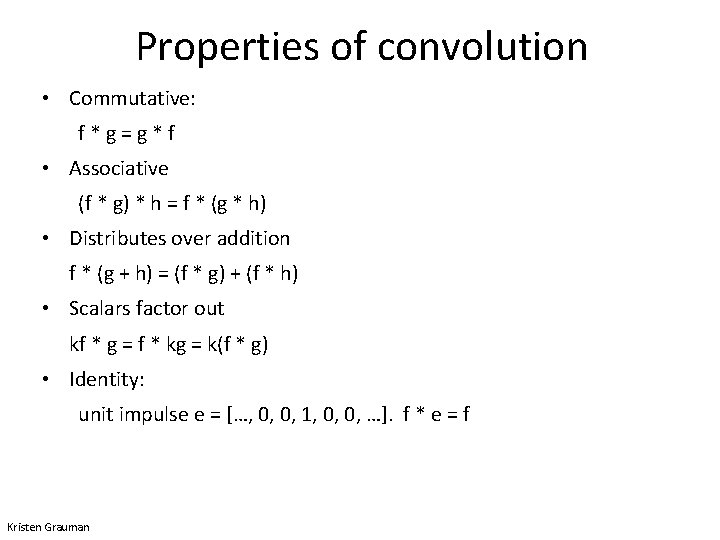
Properties of convolution • Commutative: f*g=g*f • Associative (f * g) * h = f * (g * h) • Distributes over addition f * (g + h) = (f * g) + (f * h) • Scalars factor out kf * g = f * kg = k(f * g) • Identity: unit impulse e = […, 0, 0, 1, 0, 0, …]. f * e = f Kristen Grauman

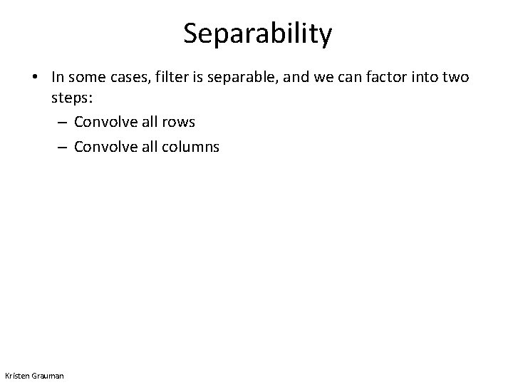
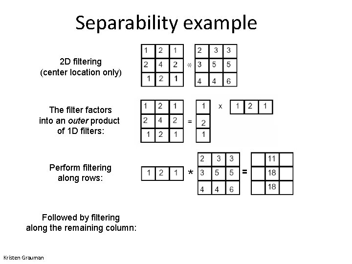
Separability • In some cases, filter is separable, and we can factor into two steps: – Convolve all rows – Convolve all columns Kristen Grauman

Separability example 2 D filtering (center location only) The filter factors into an outer product of 1 D filters: Perform filtering along rows: Followed by filtering along the remaining column: Kristen Grauman * =

Plan for today • Filters: math and properties • Types of filters – Linear • Smoothing • Other – Non-linear • Median • Texture representation with filters

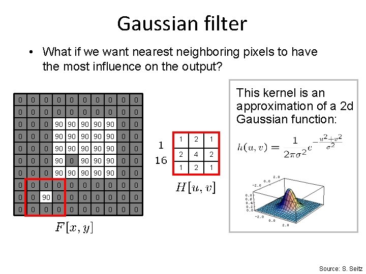
Gaussian filter • What if we want nearest neighboring pixels to have the most influence on the output? 0 0 0 0 0 0 90 90 90 0 0 90 90 90 0 90 90 90 0 0 0 0 0 0 0 0 0 0 This kernel is an approximation of a 2 d Gaussian function: 1 2 4 2 1 Source: S. Seitz

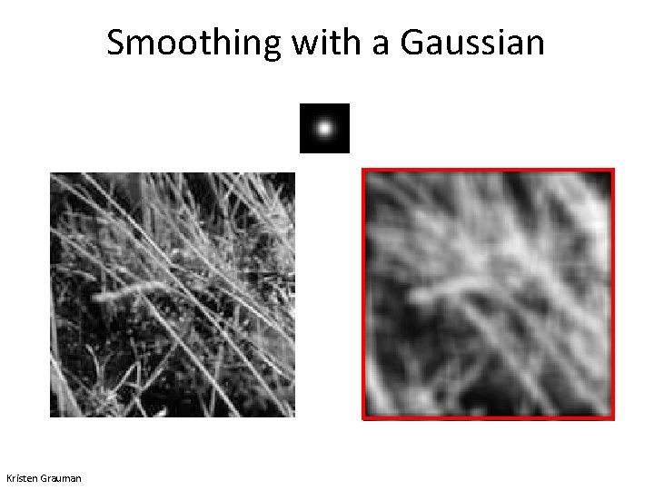
Smoothing with a Gaussian Kristen Grauman

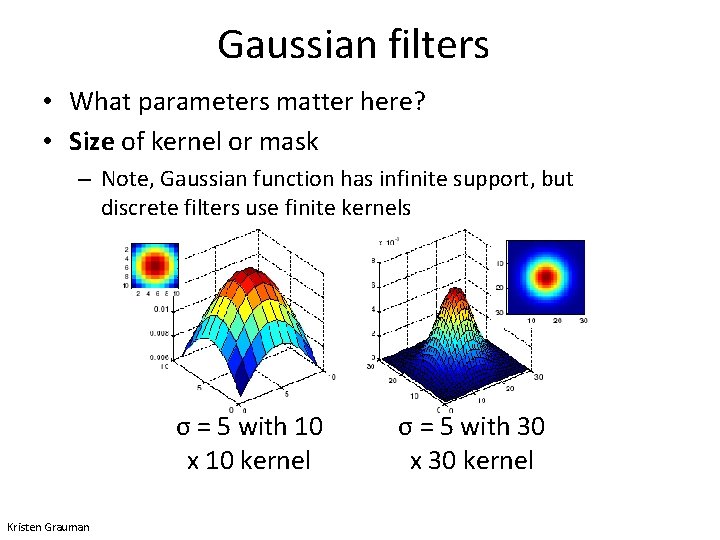
Gaussian filters • What parameters matter here? • Size of kernel or mask – Note, Gaussian function has infinite support, but discrete filters use finite kernels σ = 5 with 10 x 10 kernel Kristen Grauman σ = 5 with 30 x 30 kernel

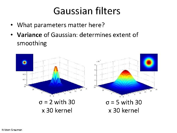
Gaussian filters • What parameters matter here? • Variance of Gaussian: determines extent of smoothing σ = 2 with 30 x 30 kernel Kristen Grauman σ = 5 with 30 x 30 kernel

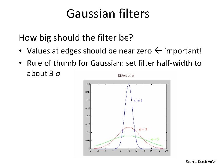
Gaussian filters How big should the filter be? • Values at edges should be near zero important! • Rule of thumb for Gaussian: set filter half-width to about 3 σ Source: Derek Hoiem

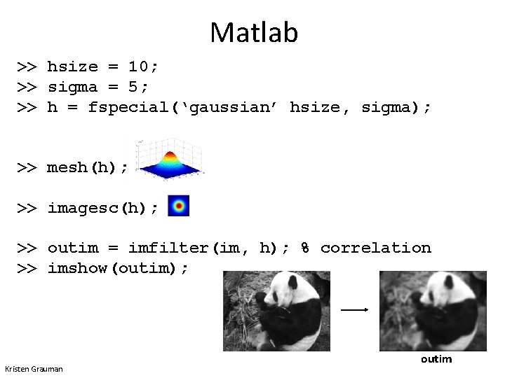
Matlab >> hsize = 10; >> sigma = 5; >> h = fspecial(‘gaussian’ hsize, sigma); >> mesh(h); >> imagesc(h); >> outim = imfilter(im, h); % correlation >> imshow(outim); Kristen Grauman outim

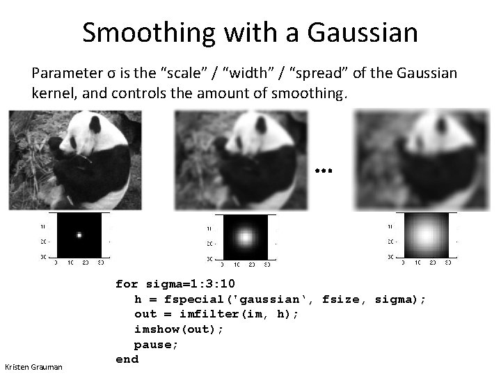
Smoothing with a Gaussian Parameter σ is the “scale” / “width” / “spread” of the Gaussian kernel, and controls the amount of smoothing. … Kristen Grauman for sigma=1: 3: 10 h = fspecial('gaussian‘, fsize, sigma); out = imfilter(im, h); imshow(out); pause; end

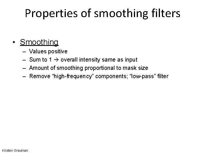
Properties of smoothing filters • Smoothing – – Kristen Grauman Values positive Sum to 1 overall intensity same as input Amount of smoothing proportional to mask size Remove “high-frequency” components; “low-pass” filter

Plan for today • Filters: math and properties • Types of filters – Linear • Smoothing • Other – Non-linear • Median • Texture representation with filters

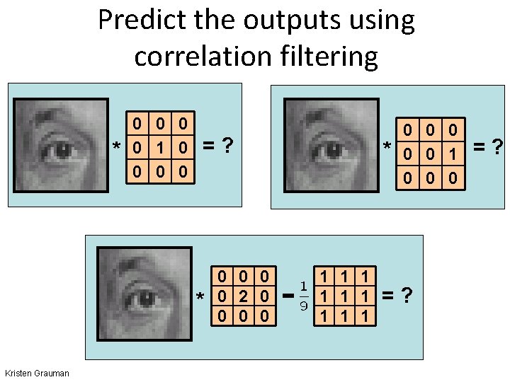
Predict the outputs using correlation filtering * 0 0 1 0 0 =? * Kristen Grauman 0 0 2 0 0 * - 1 1 1 1 1 0 0 0 =?

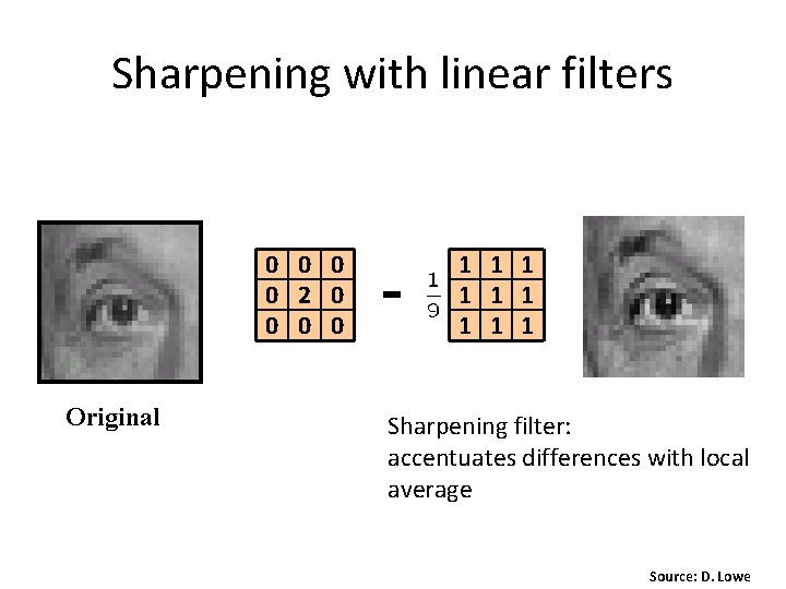
Sharpening with linear filters 0 0 2 0 0 Original - 1 1 1 1 1 Sharpening filter: accentuates differences with local average Source: D. Lowe

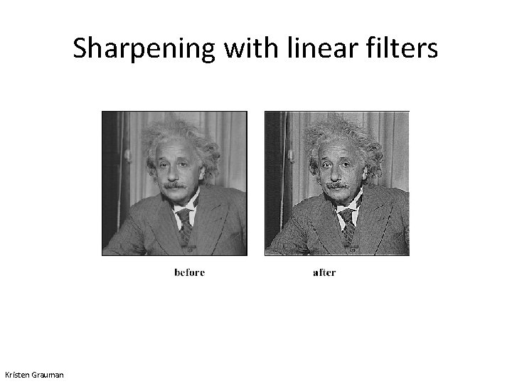
Sharpening with linear filters Kristen Grauman

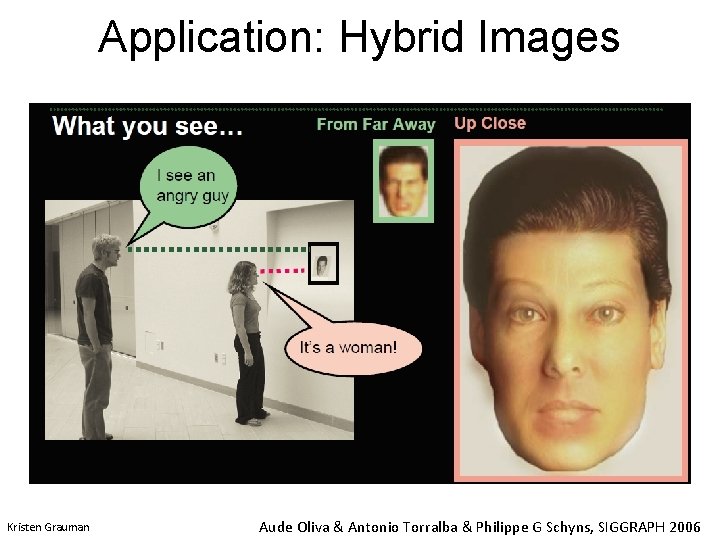
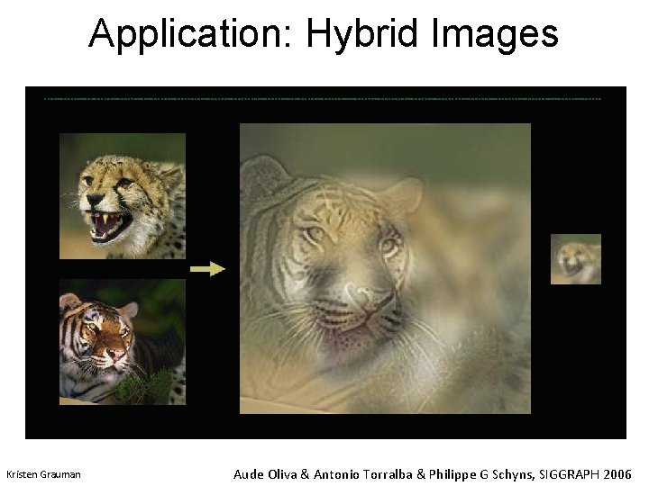
Application: Hybrid Images Kristen Grauman Aude Oliva & Antonio Torralba & Philippe G Schyns, SIGGRAPH 2006

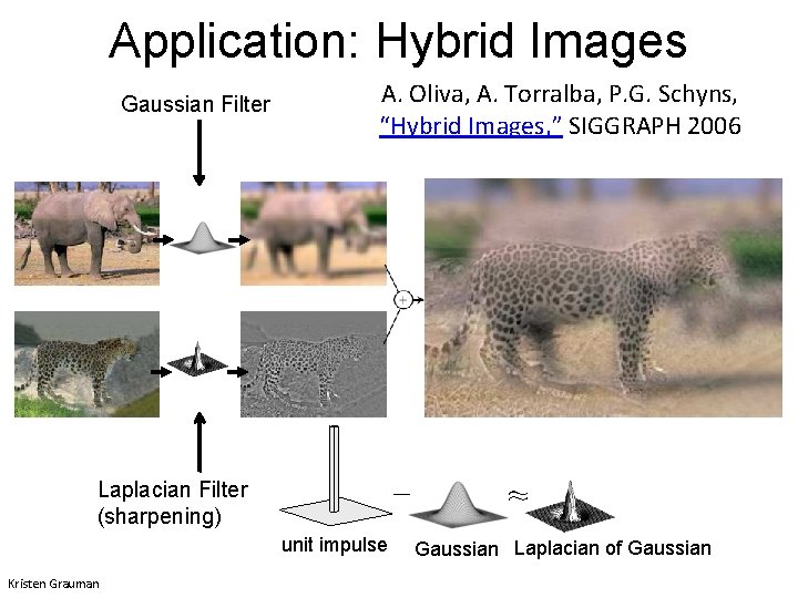
Application: Hybrid Images Gaussian Filter A. Oliva, A. Torralba, P. G. Schyns, “Hybrid Images, ” SIGGRAPH 2006 Laplacian Filter (sharpening) unit impulse Kristen Grauman Gaussian Laplacian of Gaussian

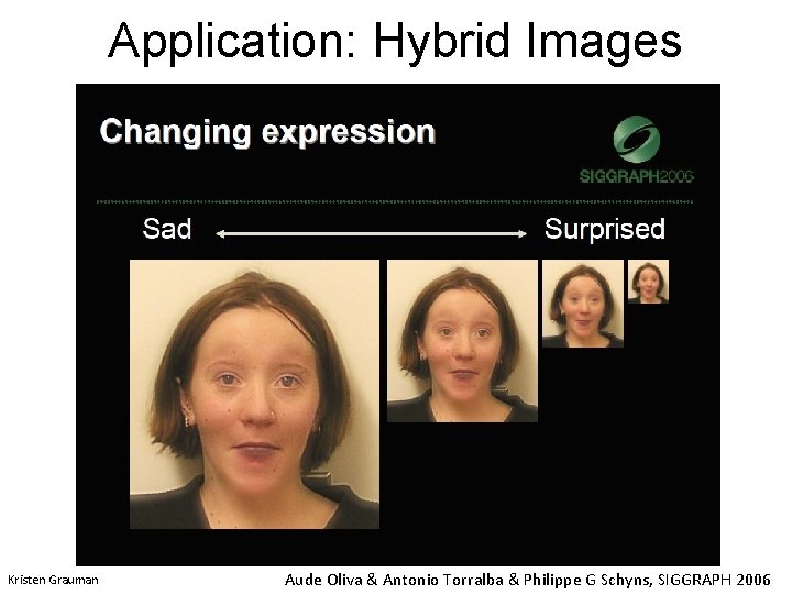
Application: Hybrid Images Kristen Grauman Aude Oliva & Antonio Torralba & Philippe G Schyns, SIGGRAPH 2006

Application: Hybrid Images Kristen Grauman Aude Oliva & Antonio Torralba & Philippe G Schyns, SIGGRAPH 2006

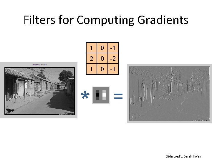
Filters for Computing Gradients * 1 0 -1 2 0 -2 1 0 -1 = Slide credit: Derek Hoiem

Plan for today • Filters: math and properties • Types of filters – Linear • Smoothing • Other – Non-linear • Median • Texture representation with filters

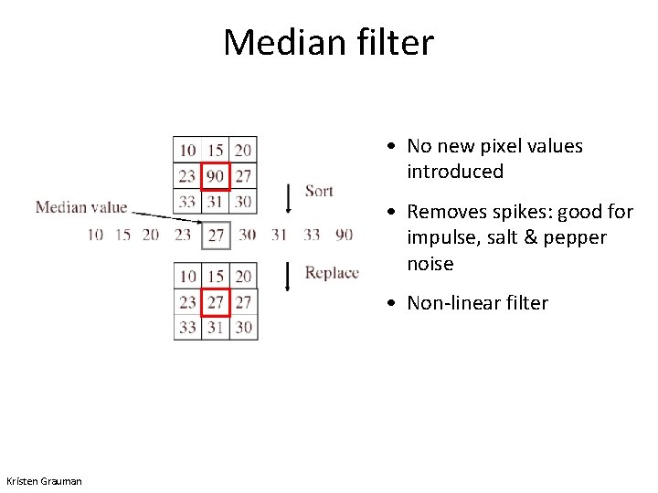
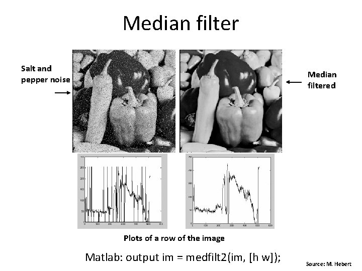
Median filter • No new pixel values introduced • Removes spikes: good for impulse, salt & pepper noise • Non-linear filter Kristen Grauman

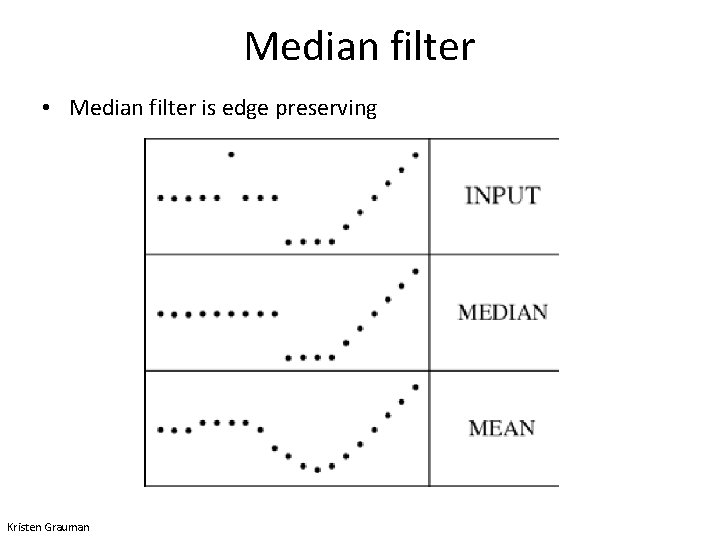
Median filter • Median filter is edge preserving Kristen Grauman

Median filter Salt and pepper noise Median filtered Plots of a row of the image Matlab: output im = medfilt 2(im, [h w]); Source: M. Hebert

1 -minute break

Plan for today • Filters: math and properties • Types of filters – Linear • Smoothing • Other – Non-linear • Median • Texture representation with filters

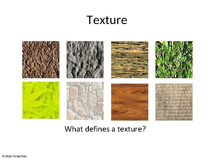
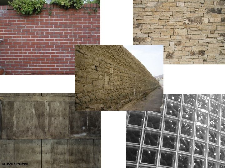
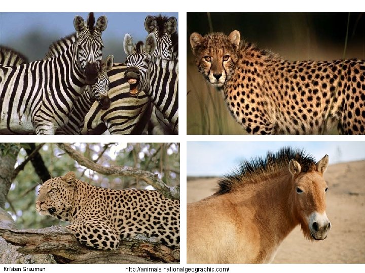
Texture What defines a texture? Kristen Grauman

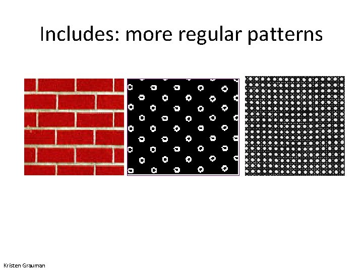
Includes: more regular patterns Kristen Grauman

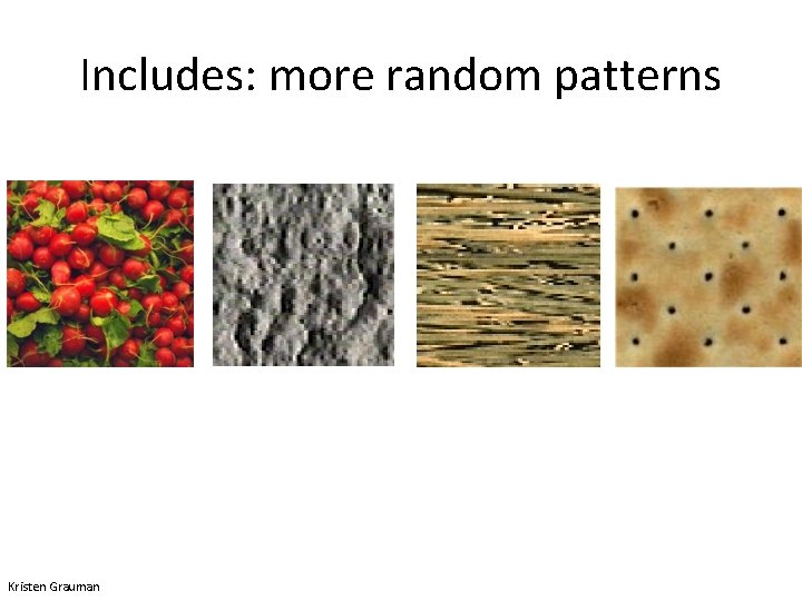
Includes: more random patterns Kristen Grauman

Kristen Grauman

Kristen Grauman http: //animals. nationalgeographic. com/

Why analyze texture? • Important for how we perceive objects • Often indicative of a material’s properties • Can be important appearance cue, especially if shape is similar across objects • To represent objects, we want a feature one step above “building blocks” of filters, edges Adapted from Kristen Grauman

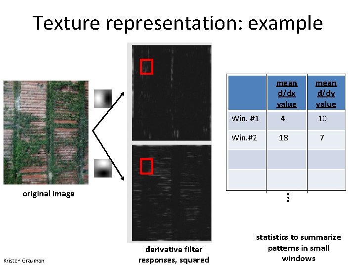
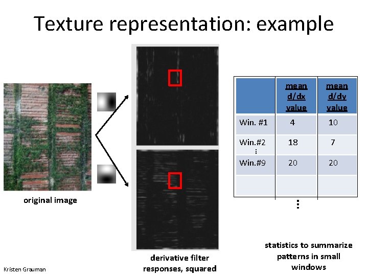
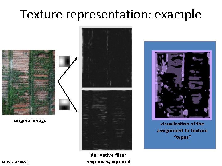
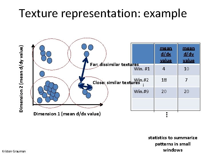
Texture representation • Textures are made up of repeated local patterns, so: – Find the patterns • Use filters that look like patterns (spots, bars, raw patches…) • Consider magnitude of response – Describe their statistics within each local window • Mean, standard deviation • Histogram Kristen Grauman

Texture representation: example mean d/dx value Win. #1 Kristen Grauman 10 … original image 4 mean d/dy value derivative filter responses, squared statistics to summarize patterns in small windows

Texture representation: example mean d/dx value Kristen Grauman Win. #1 4 10 Win. #2 18 7 … original image mean d/dy value derivative filter responses, squared statistics to summarize patterns in small windows

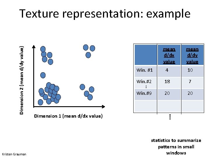
Texture representation: example mean d/dx value mean d/dy value 4 10 Win. #2 18 7 20 20 … Win. #1 Win. #9 Kristen Grauman … original image derivative filter responses, squared statistics to summarize patterns in small windows

mean d/dy value Win. #1 4 10 Win. #2 18 7 20 20 Win. #9 Dimension 1 (mean d/dx value) … Kristen Grauman mean d/dx value … Dimension 2 (mean d/dy value) Texture representation: example statistics to summarize patterns in small windows

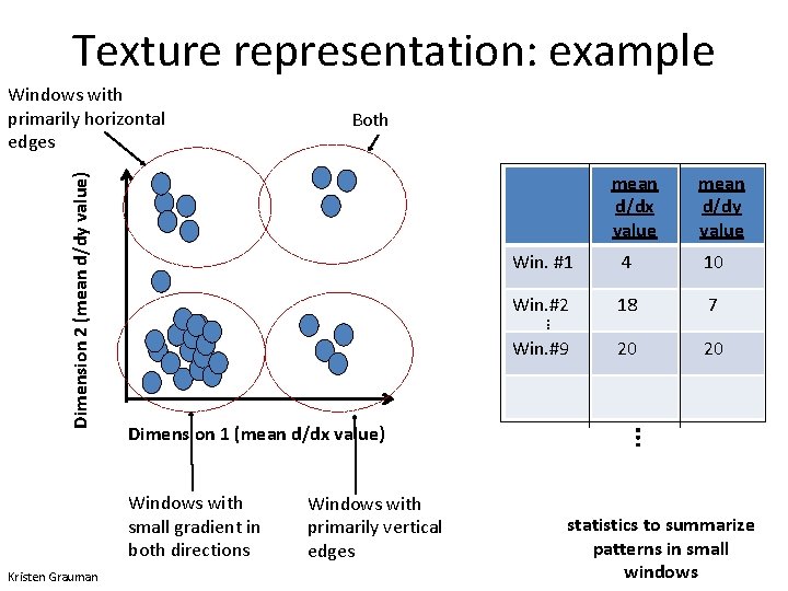
Texture representation: example mean d/dx value mean d/dy value Win. #1 4 10 Win. #2 18 7 20 20 Win. #9 Windows with primarily vertical edges … Dimension 1 (mean d/dx value) Windows with small gradient in both directions Kristen Grauman Both … Dimension 2 (mean d/dy value) Windows with primarily horizontal edges statistics to summarize patterns in small windows

Texture representation: example original image Kristen Grauman visualization of the assignment to texture “types” derivative filter responses, squared

mean d/dy value 4 10 Win. #2 Close: similar textures 18 7 Win. #9 20 20 Dimension 1 (mean d/dx value) … Kristen Grauman Far: dissimilar textures Win. #1 mean d/dx value … Dimension 2 (mean d/dy value) Texture representation: example statistics to summarize patterns in small windows

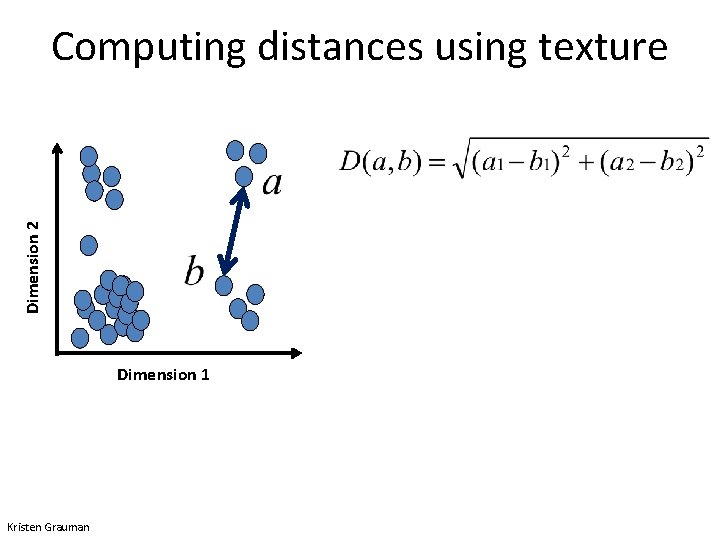
Dimension 2 Computing distances using texture Dimension 1 Kristen Grauman

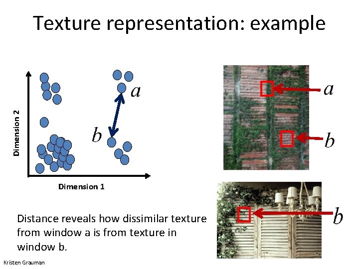
Dimension 2 Texture representation: example Dimension 1 Distance reveals how dissimilar texture from window a is from texture in window b. Kristen Grauman

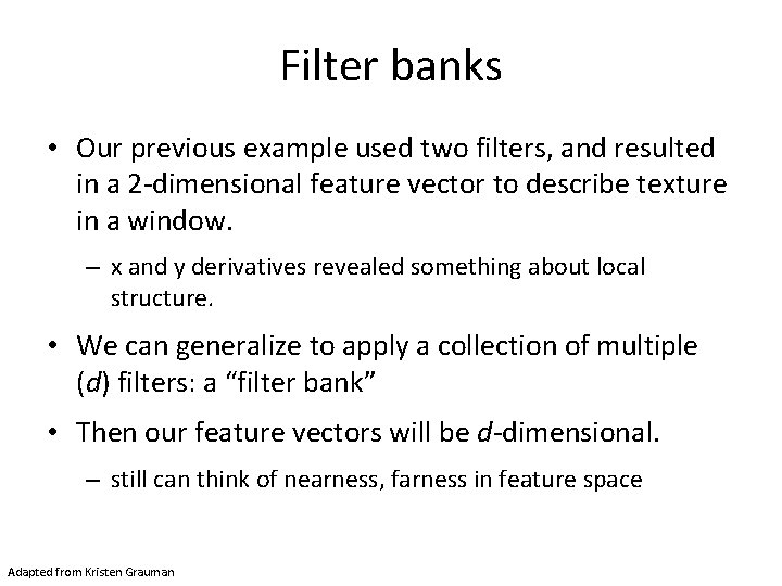
Filter banks • Our previous example used two filters, and resulted in a 2 -dimensional feature vector to describe texture in a window. – x and y derivatives revealed something about local structure. • We can generalize to apply a collection of multiple (d) filters: a “filter bank” • Then our feature vectors will be d-dimensional. – still can think of nearness, farness in feature space Adapted from Kristen Grauman

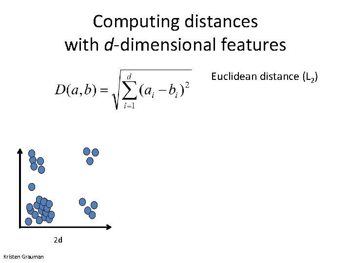
Computing distances with d-dimensional features Euclidean distance (L 2) . . . 2 d Kristen Grauman 3 d

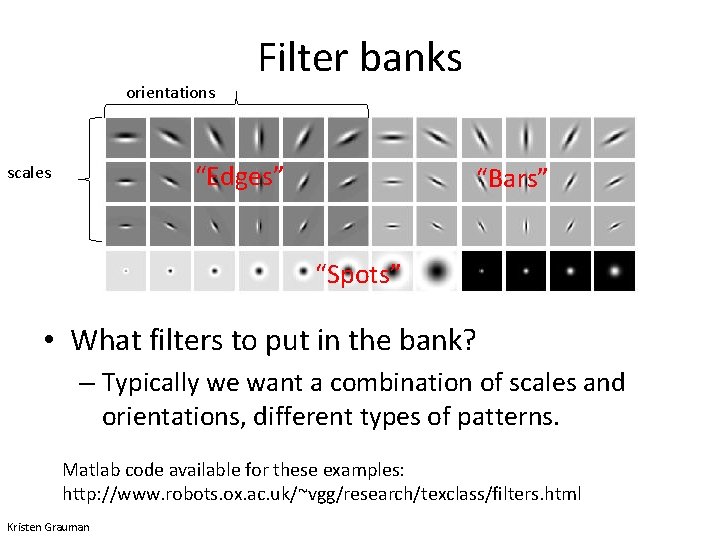
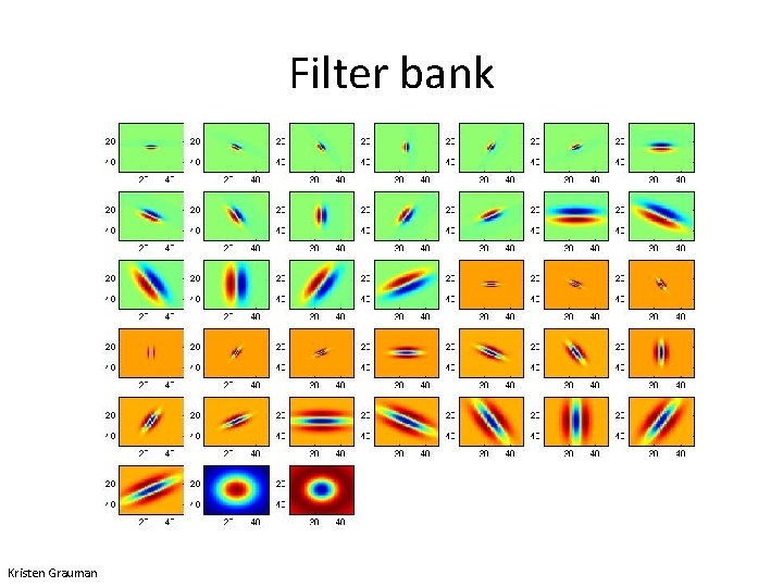
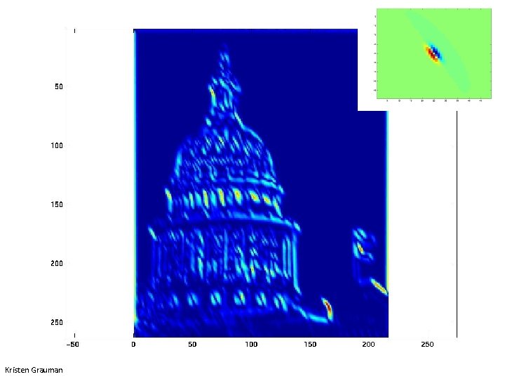
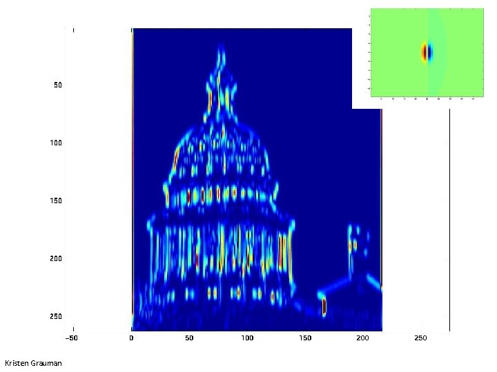
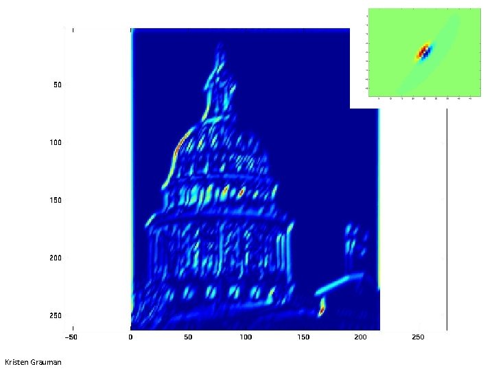
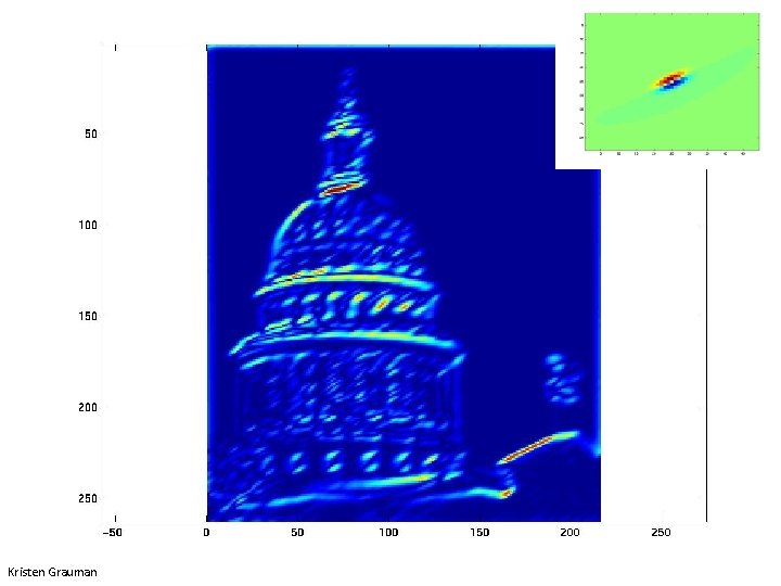
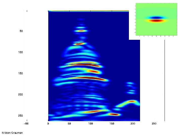
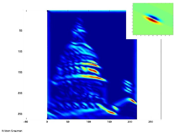
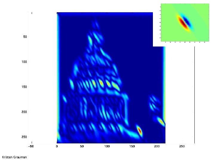
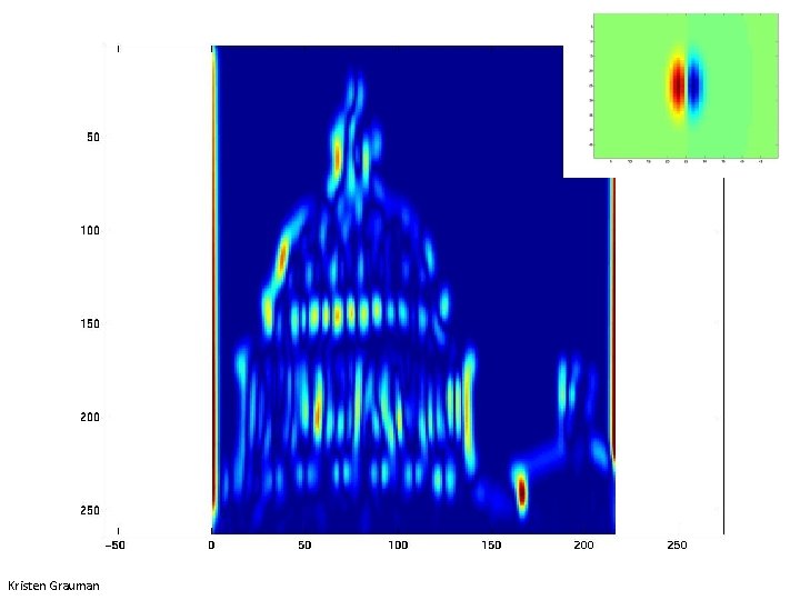
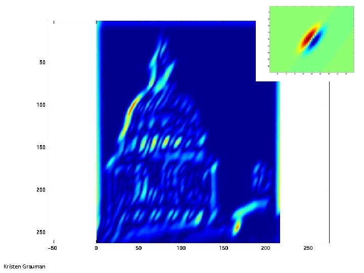
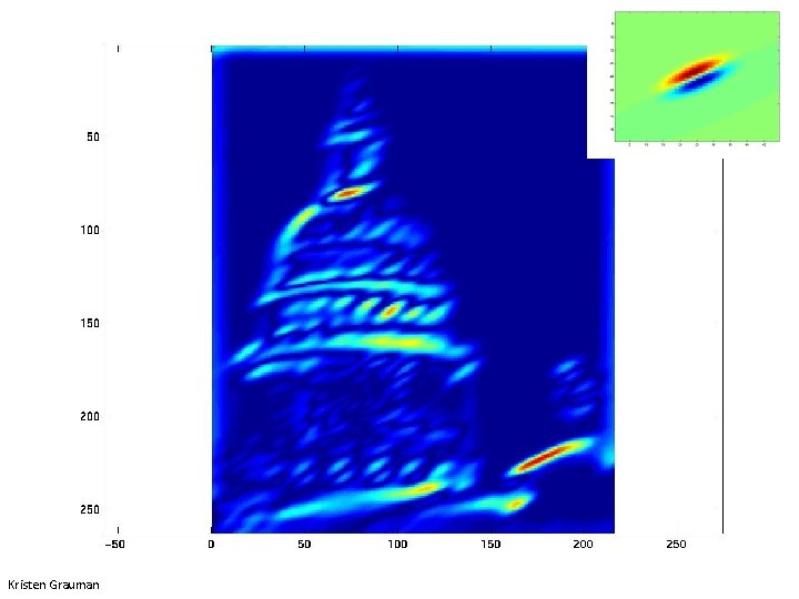
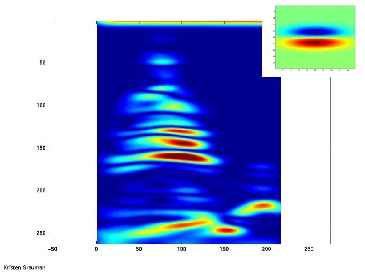
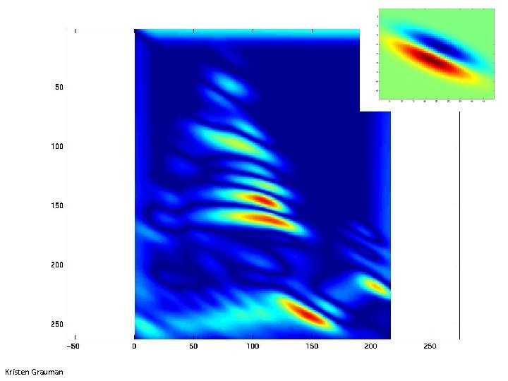
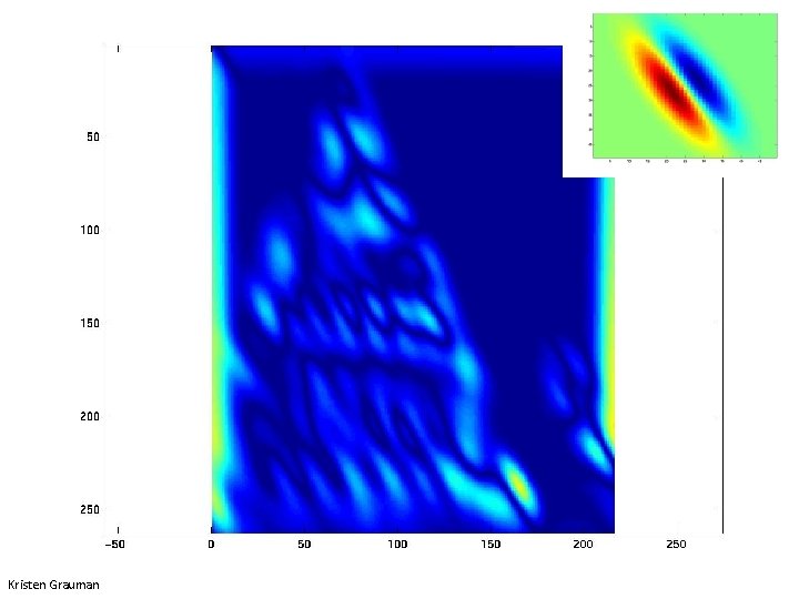
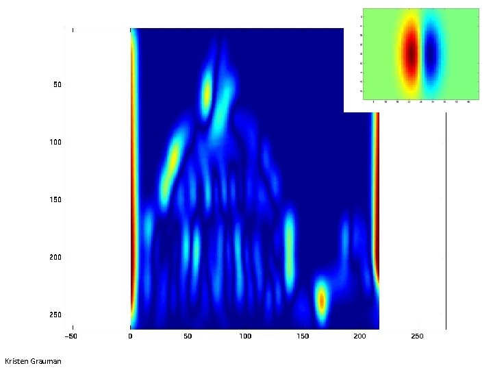
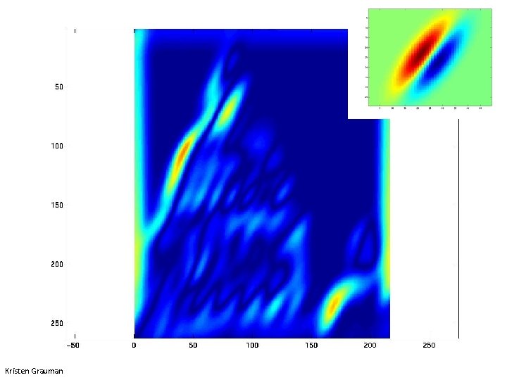
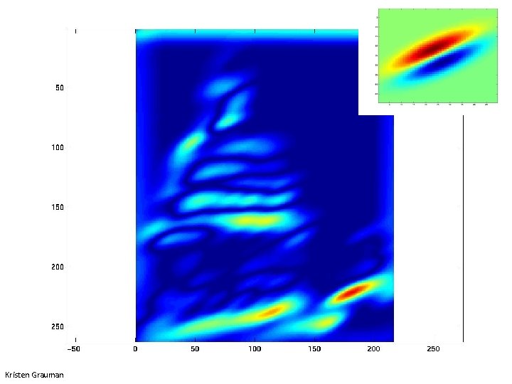
orientations Filter banks “Edges” scales “Bars” “Spots” • What filters to put in the bank? – Typically we want a combination of scales and orientations, different types of patterns. Matlab code available for these examples: http: //www. robots. ox. ac. uk/~vgg/research/texclass/filters. html Kristen Grauman

Filter bank Kristen Grauman

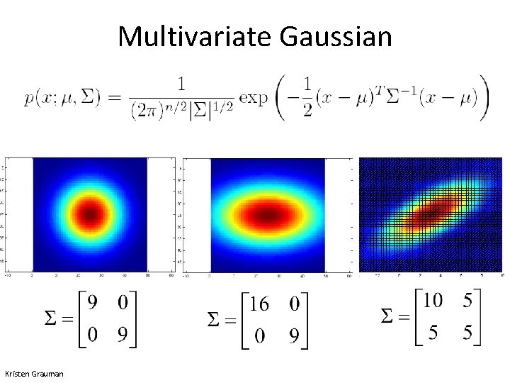
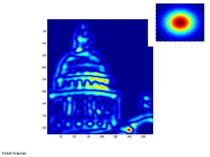
Multivariate Gaussian Kristen Grauman

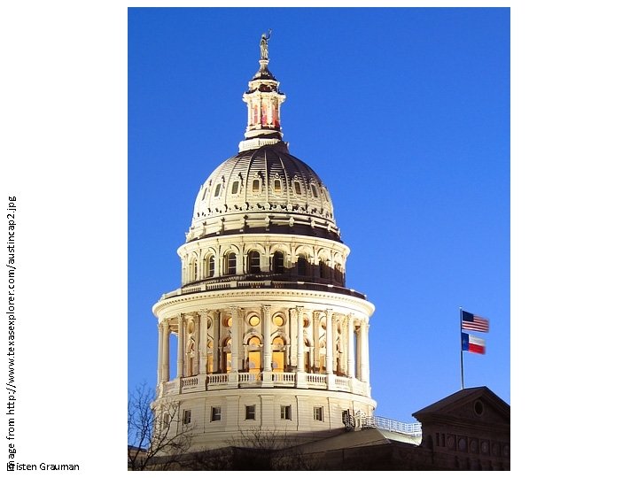
Image from http: //www. texasexplorer. com/austincap 2. jpg Kristen Grauman

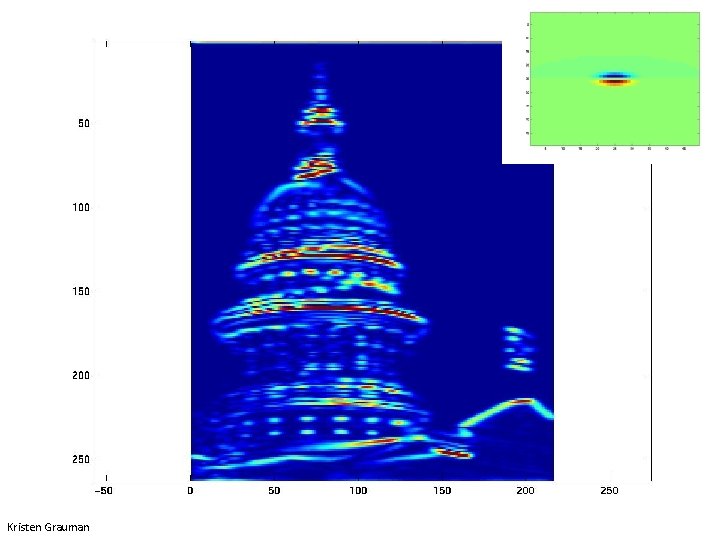
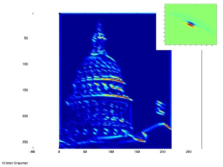
Showing magnitude of responses Kristen Grauman

Kristen Grauman

Kristen Grauman

Kristen Grauman

Kristen Grauman

Kristen Grauman

Kristen Grauman

Kristen Grauman

Kristen Grauman

Kristen Grauman

Kristen Grauman

Kristen Grauman

Kristen Grauman

Kristen Grauman

Kristen Grauman

Kristen Grauman

Kristen Grauman

Kristen Grauman

Kristen Grauman

Vectors of texture responses [r 1, r 2, …, r 38] Adapted from Kristen Grauman We can form a “feature vector” from the list of responses at each pixel; gives us a representation of the pixel, image.

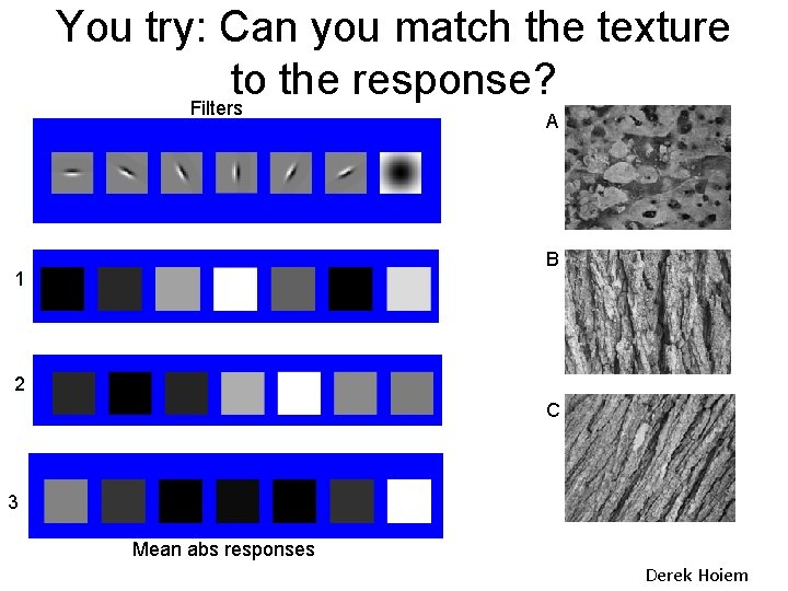
You try: Can you match the texture to the response? Filters A B 1 2 C 3 Mean abs responses Derek Hoiem

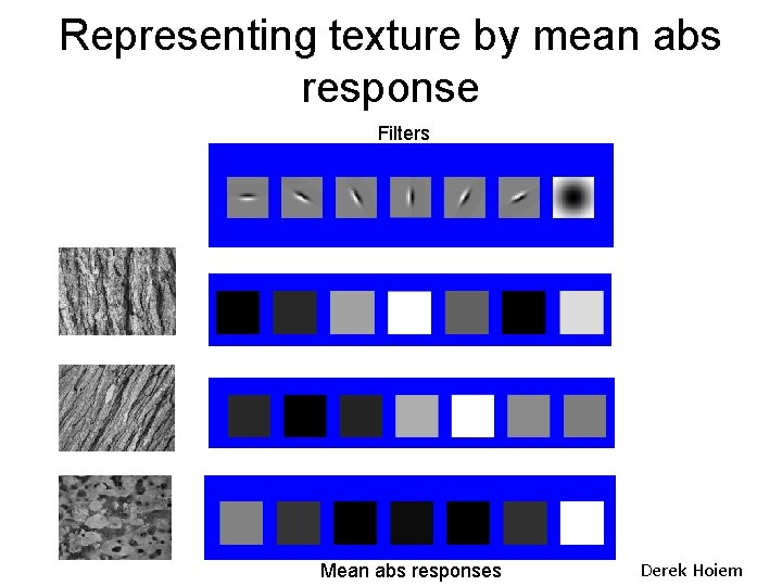
Representing texture by mean abs response Filters Mean abs responses Derek Hoiem

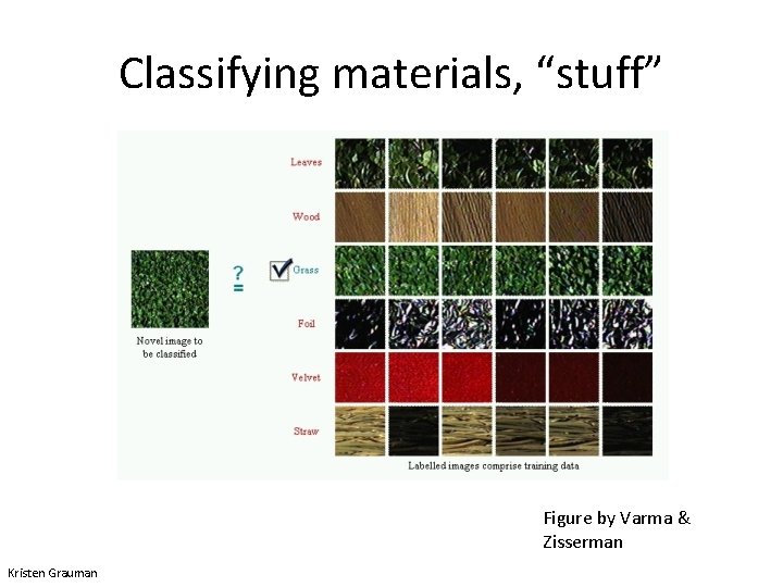
Classifying materials, “stuff” Figure by Varma & Zisserman Kristen Grauman

Summary • Filters useful for – Enhancing images (smoothing, removing noise), e. g. • Box filter (linear) • Gaussian filter (linear) • Median filter – Detecting patterns (e. g. gradients) • Texture is a useful property that is often indicative of materials, appearance cues – Texture representations attempt to summarize repeating patterns of local structure – Filter banks useful to measure redundant variety of structures in local neighborhood