CS 1674 Intro to Computer Vision Grouping Edges

CS 1674: Intro to Computer Vision Grouping: Edges, Lines, Circles, Segments Prof. Adriana Kovashka University of Pittsburgh February 8, 2018

Plan for today • Edges – Extract gradients and threshold • Lines – Find which edge points are collinear or belong to another shape e. g. circle – Automatically detect and ignore outliers • Segments – Find which pixels form a consistent region – Clustering (e. g. K-means)

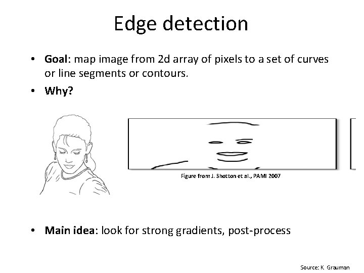
Edge detection • Goal: map image from 2 d array of pixels to a set of curves or line segments or contours. • Why? Figure from J. Shotton et al. , PAMI 2007 • Main idea: look for strong gradients, post-process Source: K. Grauman

Designing an edge detector • Criteria for a good edge detector: – Good detection: find all real edges, ignoring noise or other artifacts – Good localization • detect edges as close as possible to the true edges • return one point only for each true edge point • Cues of edge detection – Differences in color, intensity, or texture across the boundary – Continuity and closure – High-level knowledge Source: L. Fei-Fei

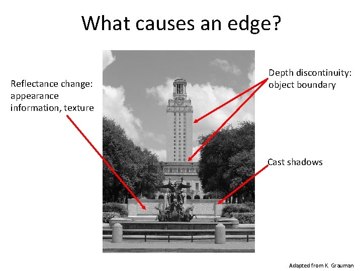
What causes an edge? Reflectance change: appearance information, texture Depth discontinuity: object boundary Cast shadows Adapted from K. Grauman

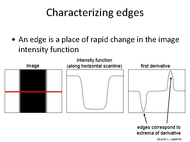
Characterizing edges • An edge is a place of rapid change in the image intensity function (along horizontal scanline) first derivative edges correspond to extrema of derivative Source: L. Lazebnik

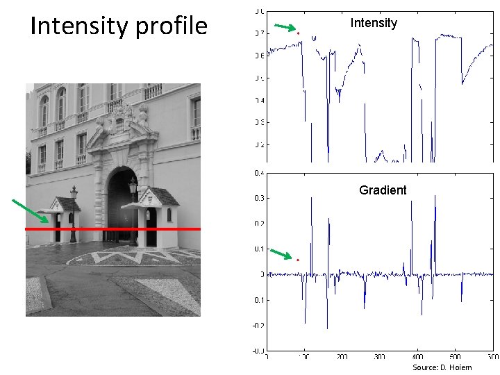
Intensity profile Intensity Gradient Source: D. Hoiem

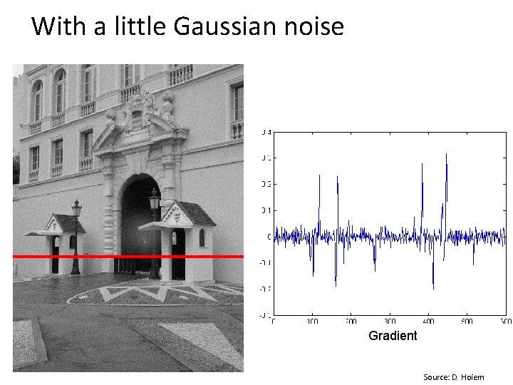
With a little Gaussian noise Gradient Source: D. Hoiem

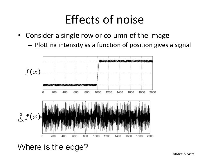
Effects of noise • Consider a single row or column of the image – Plotting intensity as a function of position gives a signal Where is the edge? Source: S. Seitz

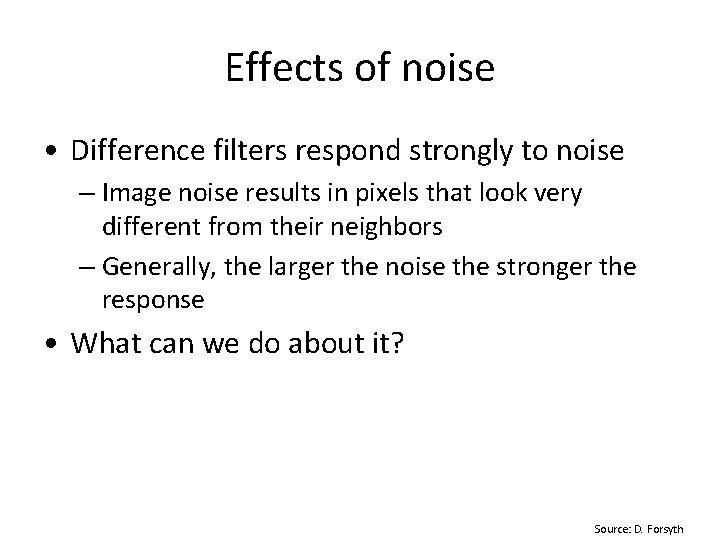
Effects of noise • Difference filters respond strongly to noise – Image noise results in pixels that look very different from their neighbors – Generally, the larger the noise the stronger the response • What can we do about it? Source: D. Forsyth

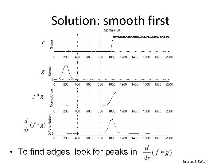
Solution: smooth first f g f*g • To find edges, look for peaks in Source: S. Seitz

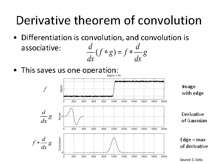
Derivative theorem of convolution • Differentiation is convolution, and convolution is associative: • This saves us one operation: f Image with edge Derivative of Gaussian Edge = max of derivative Source: S. Seitz

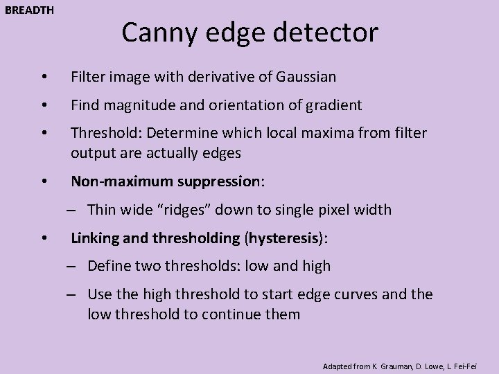
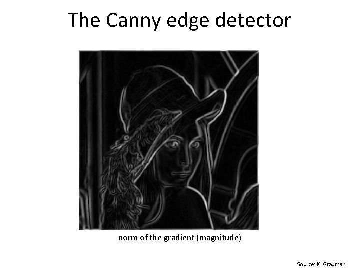
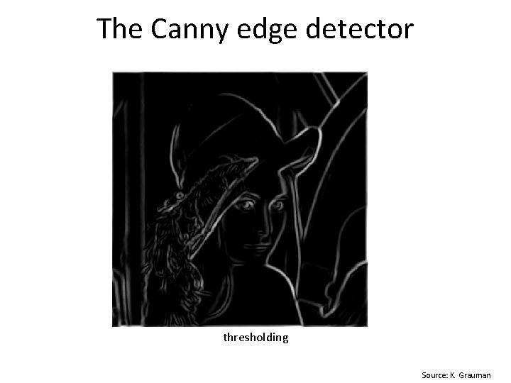
BREADTH Canny edge detector • Filter image with derivative of Gaussian • Find magnitude and orientation of gradient • Threshold: Determine which local maxima from filter output are actually edges • Non-maximum suppression: – Thin wide “ridges” down to single pixel width • Linking and thresholding (hysteresis): – Define two thresholds: low and high – Use the high threshold to start edge curves and the low threshold to continue them Adapted from K. Grauman, D. Lowe, L. Fei-Fei

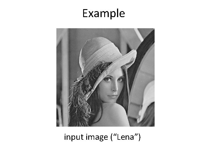
Example input image (“Lena”)

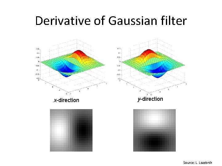
Derivative of Gaussian filter x-direction y-direction Source: L. Lazebnik

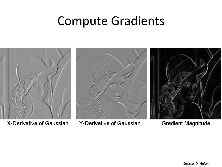
Compute Gradients X-Derivative of Gaussian Y-Derivative of Gaussian Gradient Magnitude Source: D. Hoiem

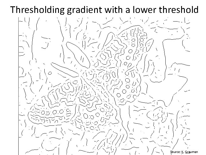
Thresholding • Choose a threshold value t • Set any pixels less than t to 0 (off) • Set any pixels greater than or equal to t to 1 (on) Source: K. Grauman

The Canny edge detector norm of the gradient (magnitude) Source: K. Grauman

The Canny edge detector thresholding Source: K. Grauman

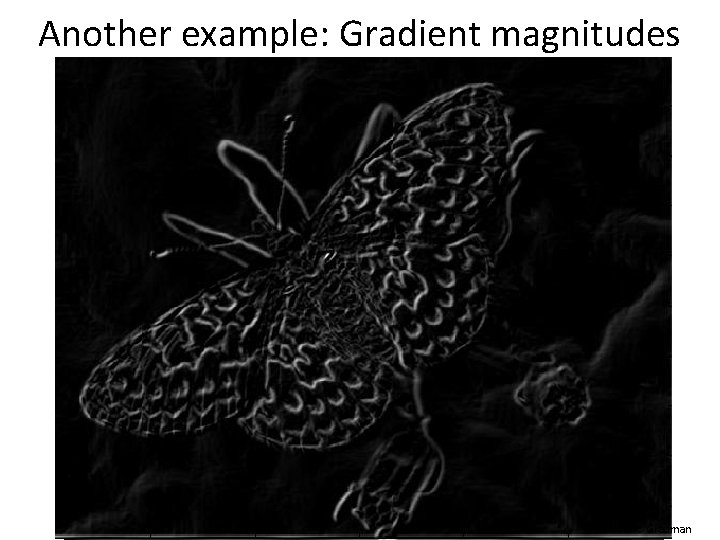
Another example: Gradient magnitudes Source: K. Grauman

Thresholding gradient with a lower threshold Source: K. Grauman

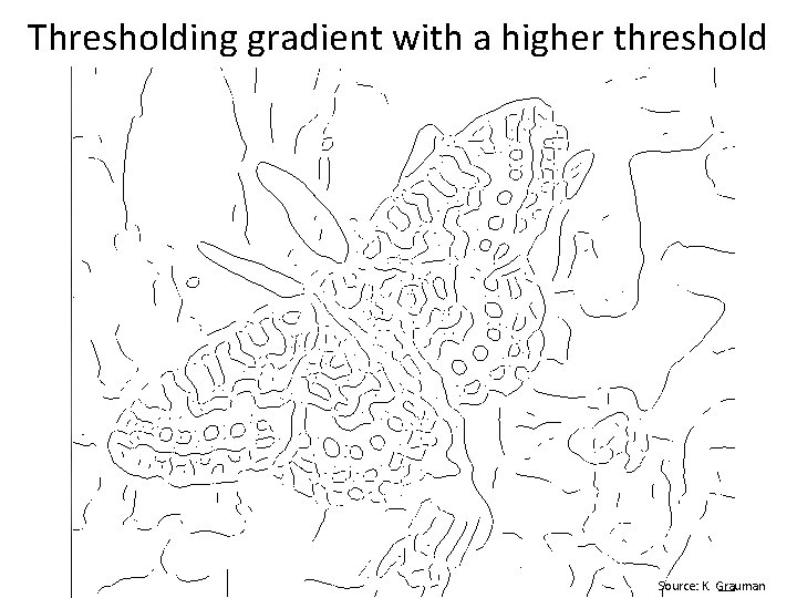
Thresholding gradient with a higher threshold Source: K. Grauman

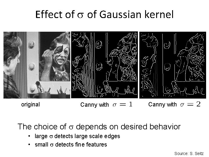
Effect of Gaussian kernel original Canny with The choice of depends on desired behavior • large detects large scale edges • small detects fine features Source: S. Seitz

Plan for today • Edges – Extract gradients and threshold • Lines – Find which edge points are collinear or belong to another shape e. g. circle – Automatically detect and ignore outliers • Segments – Find which pixels form a consistent region – Clustering (e. g. K-means)

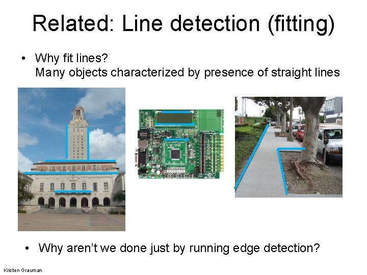
Related: Line detection (fitting) • Why fit lines? Many objects characterized by presence of straight lines • Why aren’t we done just by running edge detection? Kristen Grauman

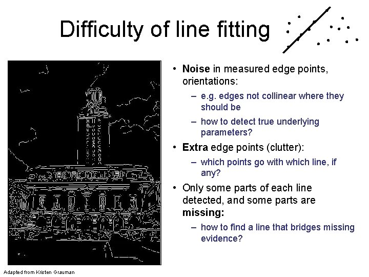
Difficulty of line fitting • Noise in measured edge points, orientations: – e. g. edges not collinear where they should be – how to detect true underlying parameters? • Extra edge points (clutter): – which points go with which line, if any? • Only some parts of each line detected, and some parts are missing: – how to find a line that bridges missing evidence? Adapted from Kristen Grauman

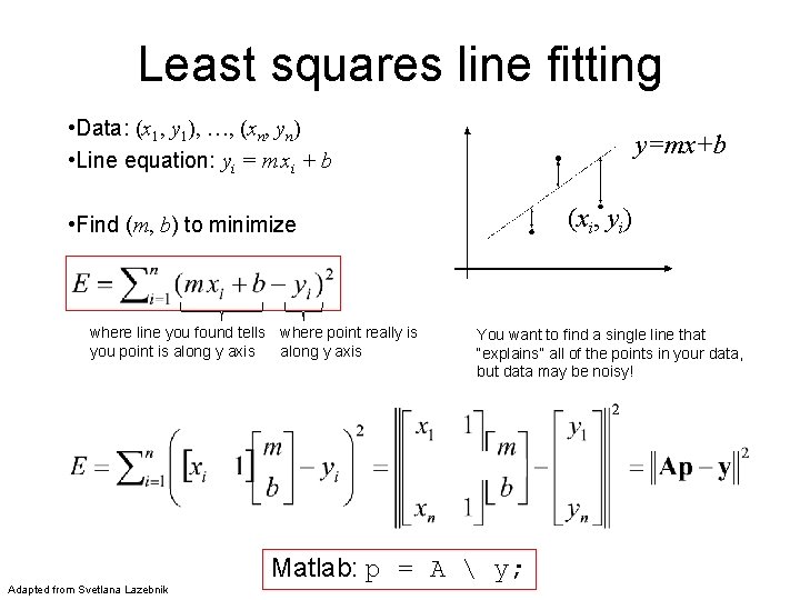
Least squares line fitting • Data: (x 1, y 1), …, (xn, yn) • Line equation: yi = m xi + b y=mx+b (xi, yi) • Find (m, b) to minimize where line you found tells where point really is you point is along y axis Adapted from Svetlana Lazebnik You want to find a single line that “explains” all of the points in your data, but data may be noisy! Matlab: p = A y;

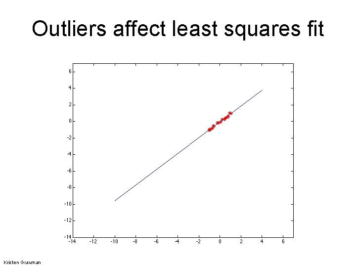
Outliers affect least squares fit Kristen Grauman

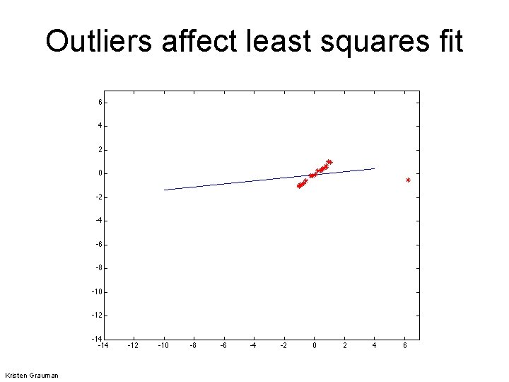
Outliers affect least squares fit Kristen Grauman

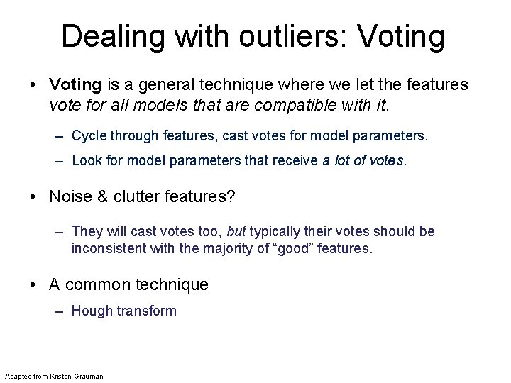
Dealing with outliers: Voting • Voting is a general technique where we let the features vote for all models that are compatible with it. – Cycle through features, cast votes for model parameters. – Look for model parameters that receive a lot of votes. • Noise & clutter features? – They will cast votes too, but typically their votes should be inconsistent with the majority of “good” features. • A common technique – Hough transform Adapted from Kristen Grauman

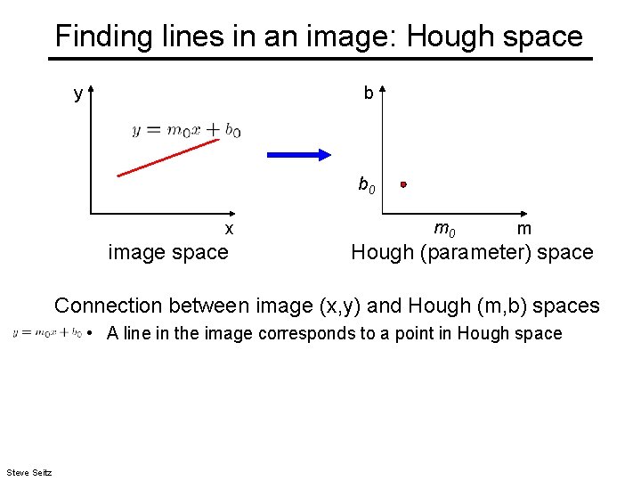
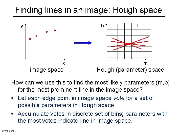
Finding lines in an image: Hough space y b b 0 x image space m 0 m Hough (parameter) space Connection between image (x, y) and Hough (m, b) spaces • A line in the image corresponds to a point in Hough space Steve Seitz

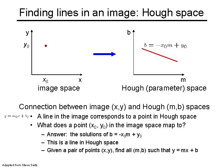
Finding lines in an image: Hough space y b y 0 x image space m Hough (parameter) space Connection between image (x, y) and Hough (m, b) spaces • A line in the image corresponds to a point in Hough space • What does a point (x 0, y 0) in the image space map to? – Answer: the solutions of b = -x 0 m + y 0 – This is a line in Hough space – Given a pair of points (x, y), find all (m, b) such that y = mx + b Adapted from Steve Seitz

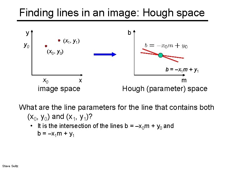
Finding lines in an image: Hough space y y 0 b (x 1, y 1) (x 0, y 0) b = –x 1 m + y 1 x 0 x image space m Hough (parameter) space What are the line parameters for the line that contains both (x 0, y 0) and (x 1, y 1)? • It is the intersection of the lines b = –x 0 m + y 0 and b = –x 1 m + y 1 Steve Seitz

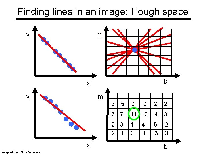
Finding lines in an image: Hough space y b x image space m Hough (parameter) space How can we use this to find the most likely parameters (m, b) for the most prominent line in the image space? • Let each edge point in image space vote for a set of possible parameters in Hough space • Accumulate votes in discrete set of bins; parameters with the most votes indicate line in image space. Steve Seitz

Finding lines in an image: Hough space y m b x y m 3 x Adapted from Silvio Savarese 5 3 3 2 2 3 7 11 10 4 3 2 1 1 0 5 3 2 3 4 1 b

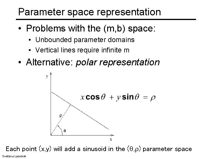
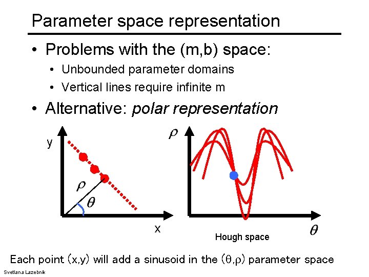
Parameter space representation • Problems with the (m, b) space: • Unbounded parameter domains • Vertical lines require infinite m • Alternative: polar representation Each point (x, y) will add a sinusoid in the ( , ) parameter space Svetlana Lazebnik

Parameter space representation • Problems with the (m, b) space: • Unbounded parameter domains • Vertical lines require infinite m • Alternative: polar representation y x Hough space Each point (x, y) will add a sinusoid in the ( , ) parameter space Svetlana Lazebnik

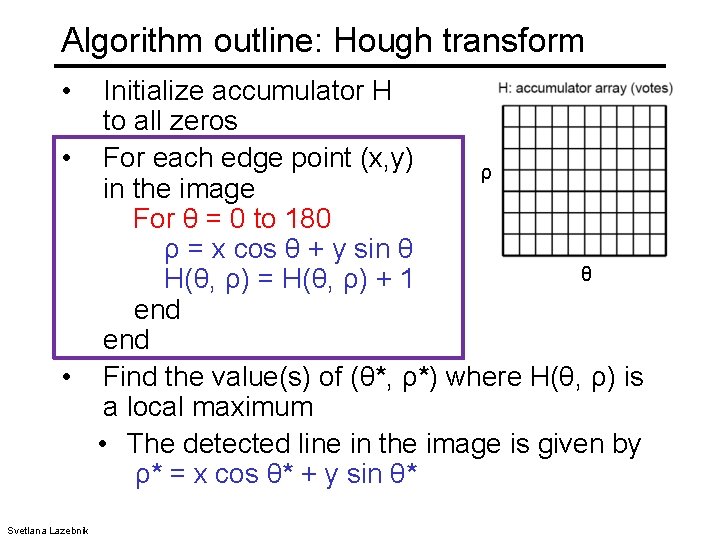
Algorithm outline: Hough transform • Initialize accumulator H to all zeros • For each edge point (x, y) ρ in the image For θ = 0 to 180 ρ = x cos θ + y sin θ θ H(θ, ρ) = H(θ, ρ) + 1 end • Find the value(s) of (θ*, ρ*) where H(θ, ρ) is a local maximum • The detected line in the image is given by ρ* = x cos θ* + y sin θ* Svetlana Lazebnik

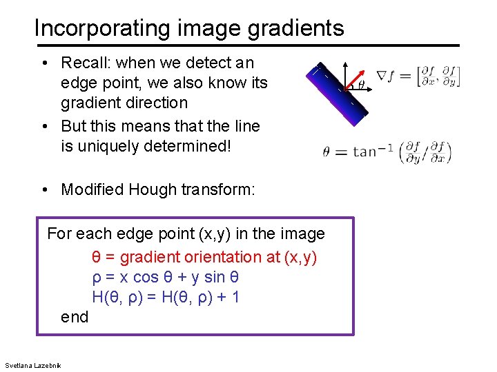
Incorporating image gradients • Recall: when we detect an edge point, we also know its gradient direction • But this means that the line is uniquely determined! • Modified Hough transform: For each edge point (x, y) in the image θ = gradient orientation at (x, y) ρ = x cos θ + y sin θ H(θ, ρ) = H(θ, ρ) + 1 end Svetlana Lazebnik

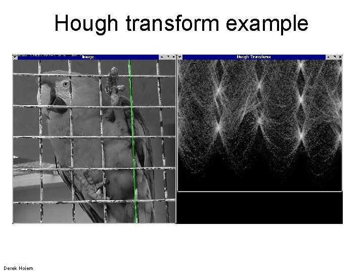
Hough transform example Derek Hoiem

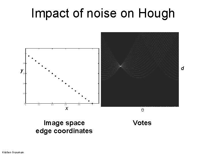
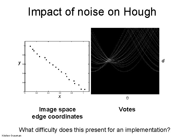
Impact of noise on Hough d y x Image space edge coordinates Kristen Grauman Votes

Impact of noise on Hough d y x Image space edge coordinates Votes What difficulty does this present for an implementation? Kristen Grauman

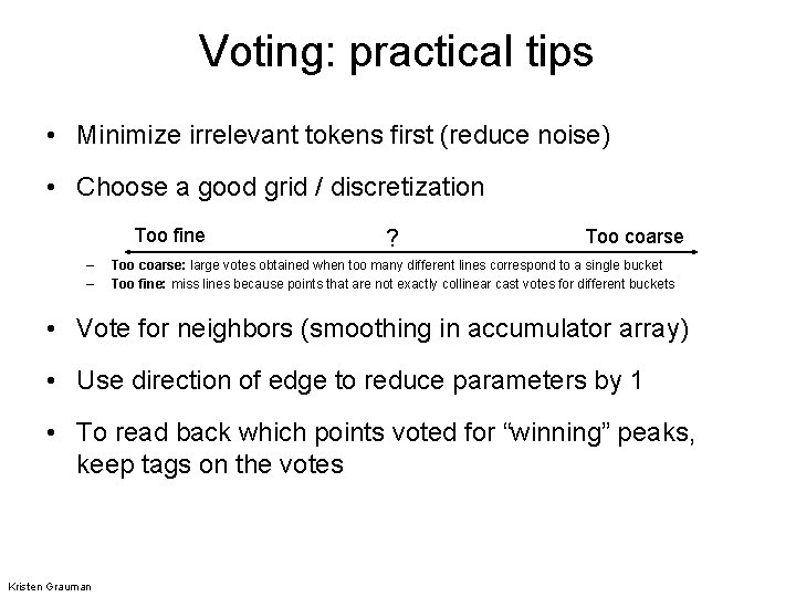
Voting: practical tips • Minimize irrelevant tokens first (reduce noise) • Choose a good grid / discretization Too fine – – ? Too coarse: large votes obtained when too many different lines correspond to a single bucket Too fine: miss lines because points that are not exactly collinear cast votes for different buckets • Vote for neighbors (smoothing in accumulator array) • Use direction of edge to reduce parameters by 1 • To read back which points voted for “winning” peaks, keep tags on the votes Kristen Grauman

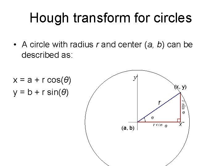
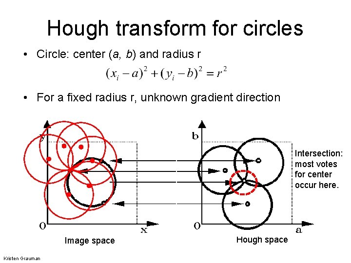
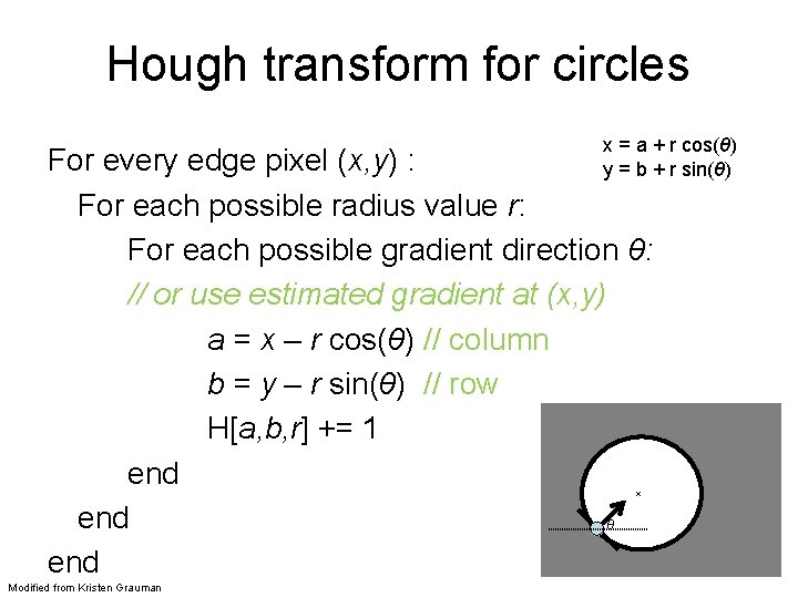
Hough transform for circles • A circle with radius r and center (a, b) can be described as: x = a + r cos(θ) y = b + r sin(θ) (x, y) ϴ ϴ (a, b) ϴ

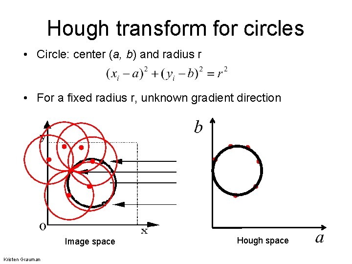
Hough transform for circles • Circle: center (a, b) and radius r • For a fixed radius r, unknown gradient direction Image space Kristen Grauman Hough space

Hough transform for circles • Circle: center (a, b) and radius r • For a fixed radius r, unknown gradient direction Intersection: most votes for center occur here. Image space Kristen Grauman Hough space

Hough transform for circles x = a + r cos(θ) y = b + r sin(θ) For every edge pixel (x, y) : For each possible radius value r: For each possible gradient direction θ: // or use estimated gradient at (x, y) a = x – r cos(θ) // column b = y – r sin(θ) // row H[a, b, r] += 1 end θ end x Modified from Kristen Grauman

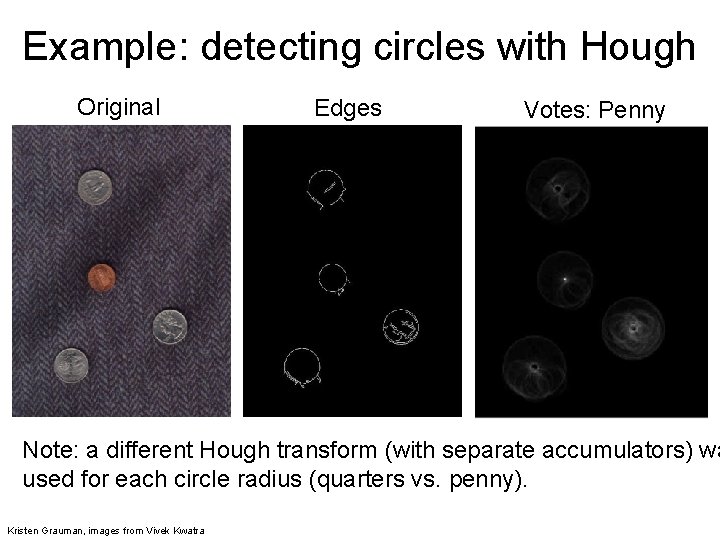
Example: detecting circles with Hough Original Edges Votes: Penny Note: a different Hough transform (with separate accumulators) wa used for each circle radius (quarters vs. penny). Kristen Grauman, images from Vivek Kwatra

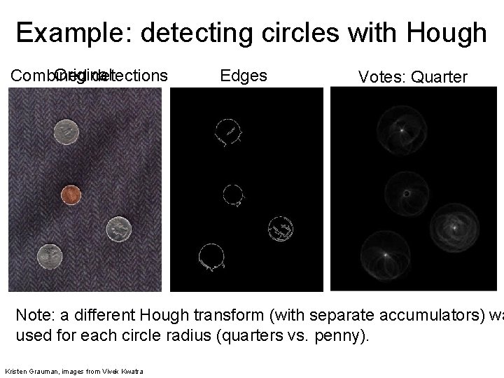
Example: detecting circles with Hough Original Combined detections Edges Votes: Quarter Note: a different Hough transform (with separate accumulators) wa used for each circle radius (quarters vs. penny). Kristen Grauman, images from Vivek Kwatra

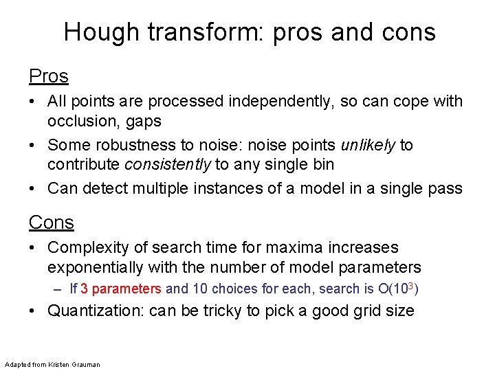
Hough transform: pros and cons Pros • All points are processed independently, so can cope with occlusion, gaps • Some robustness to noise: noise points unlikely to contribute consistently to any single bin • Can detect multiple instances of a model in a single pass Cons • Complexity of search time for maxima increases exponentially with the number of model parameters – If 3 parameters and 10 choices for each, search is O(103) • Quantization: can be tricky to pick a good grid size Adapted from Kristen Grauman

BREADTH Check hidden slides for: • Generalized Hough transform algorithm • RANSAC (another voting algorithm)

Plan for today • Edges – Extract gradients and threshold • Lines – Find which edge points are collinear or belong to another shape e. g. circle – Automatically detect and ignore outliers • Segments – Find which pixels form a consistent region – Clustering (e. g. K-means)

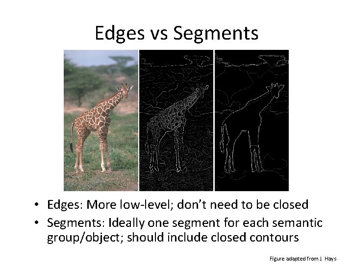
Edges vs Segments • Edges: More low-level; don’t need to be closed • Segments: Ideally one segment for each semantic group/object; should include closed contours Figure adapted from J. Hays

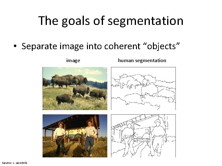
The goals of segmentation • Separate image into coherent “objects” image Source: L. Lazebnik human segmentation

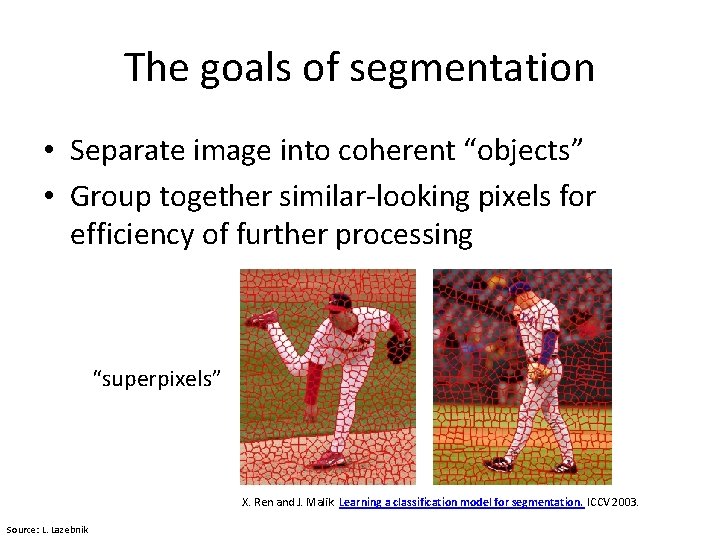
The goals of segmentation • Separate image into coherent “objects” • Group together similar-looking pixels for efficiency of further processing “superpixels” X. Ren and J. Malik. Learning a classification model for segmentation. ICCV 2003. Source: L. Lazebnik

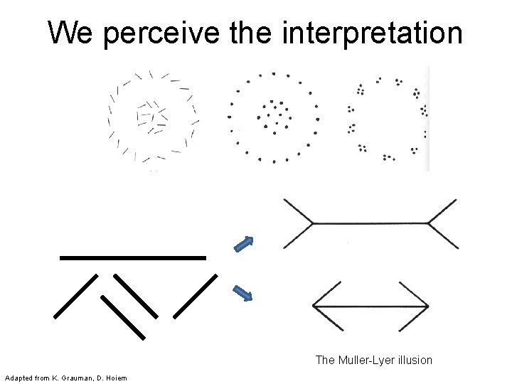
We perceive the interpretation The Muller-Lyer illusion Adapted from K. Grauman, D. Hoiem

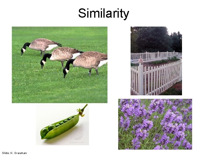
Similarity Slide: K. Grauman

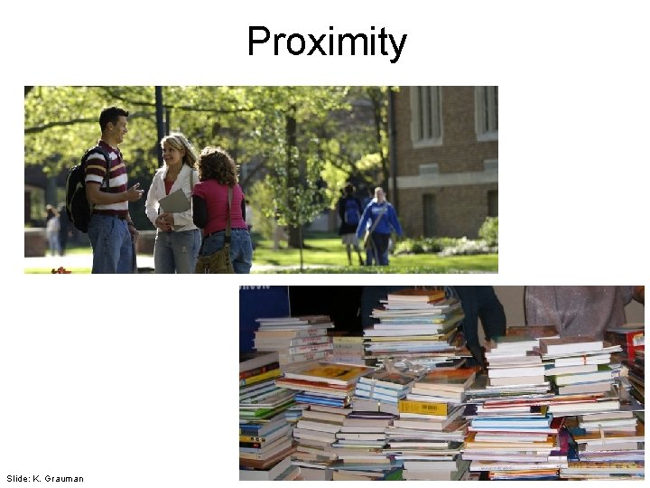
Proximity Slide: K. Grauman

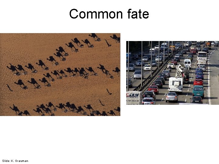
Common fate Slide: K. Grauman

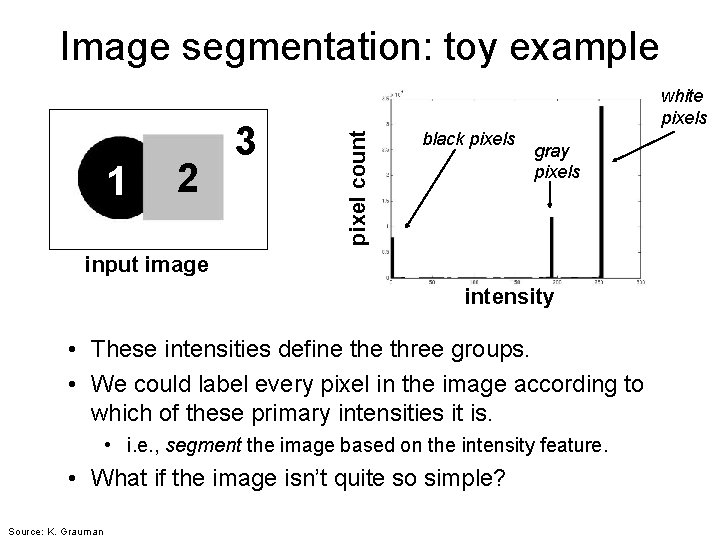
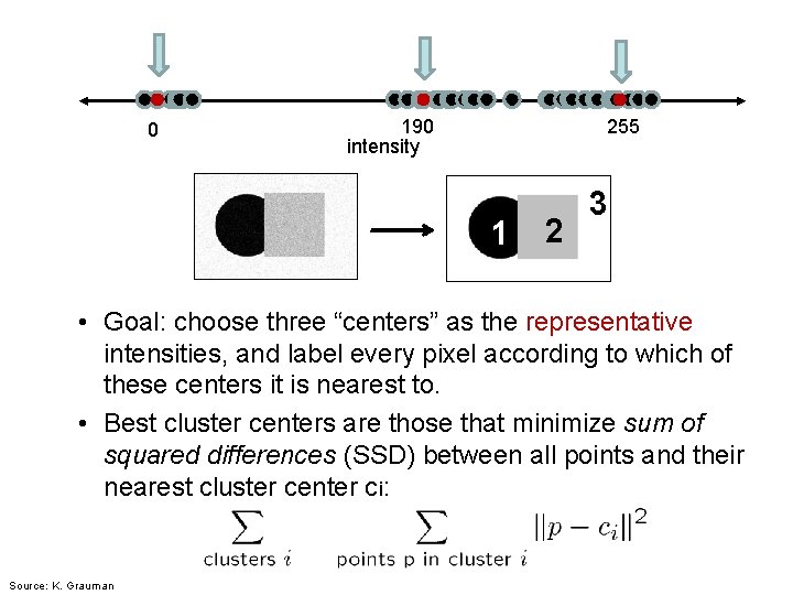
Image segmentation: toy example 2 pixel count 1 3 white pixels black pixels gray pixels input image intensity • These intensities define three groups. • We could label every pixel in the image according to which of these primary intensities it is. • i. e. , segment the image based on the intensity feature. • What if the image isn’t quite so simple? Source: K. Grauman

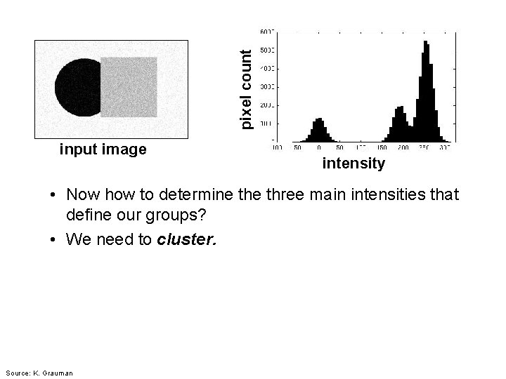
pixel count input image intensity • Now how to determine three main intensities that define our groups? • We need to cluster. Source: K. Grauman

0 190 intensity 255 1 2 3 • Goal: choose three “centers” as the representative intensities, and label every pixel according to which of these centers it is nearest to. • Best cluster centers are those that minimize sum of squared differences (SSD) between all points and their nearest cluster center ci: Source: K. Grauman

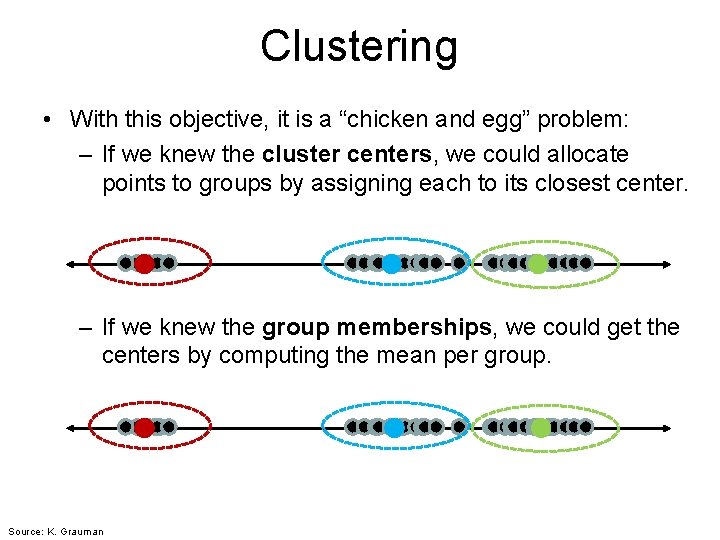
Clustering • With this objective, it is a “chicken and egg” problem: – If we knew the cluster centers, we could allocate points to groups by assigning each to its closest center. – If we knew the group memberships, we could get the centers by computing the mean per group. Source: K. Grauman

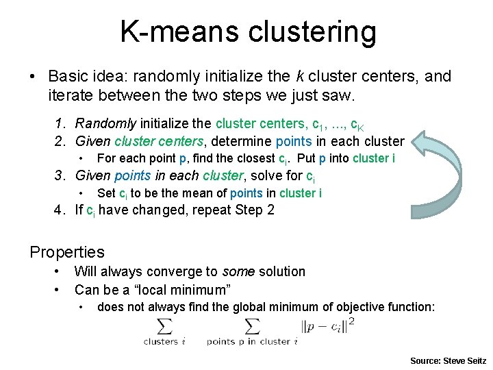
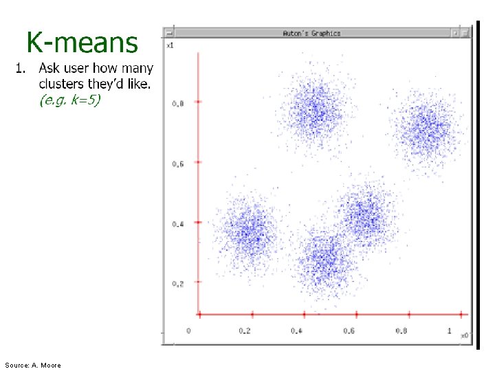
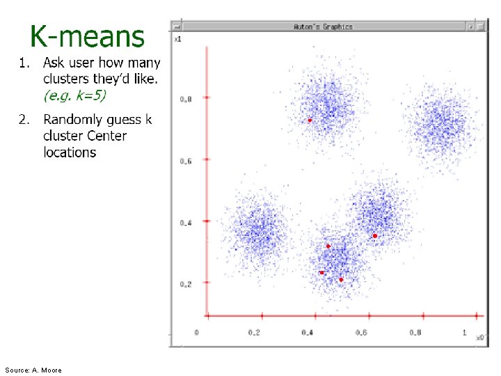
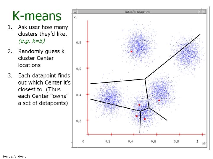
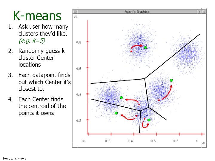
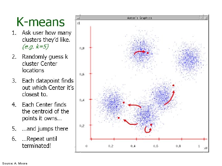
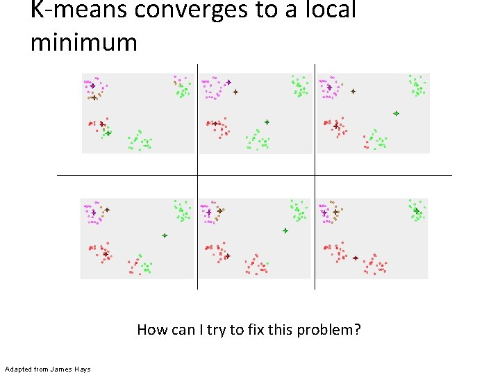
K-means clustering • Basic idea: randomly initialize the k cluster centers, and iterate between the two steps we just saw. 1. Randomly initialize the cluster centers, c 1, . . . , c. K 2. Given cluster centers, determine points in each cluster • For each point p, find the closest ci. Put p into cluster i 3. Given points in each cluster, solve for ci • Set ci to be the mean of points in cluster i 4. If ci have changed, repeat Step 2 Properties • • Will always converge to some solution Can be a “local minimum” • does not always find the global minimum of objective function: Source: Steve Seitz

Source: A. Moore

Source: A. Moore

Source: A. Moore

Source: A. Moore

Source: A. Moore

K-means converges to a local minimum How can I try to fix this problem? Adapted from James Hays

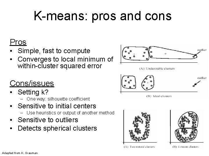
K-means: pros and cons Pros • Simple, fast to compute • Converges to local minimum of within-cluster squared error Cons/issues • Setting k? – One way: silhouette coefficient • Sensitive to initial centers – Use heuristics or output of another method • Sensitive to outliers • Detects spherical clusters Adapted from K. Grauman

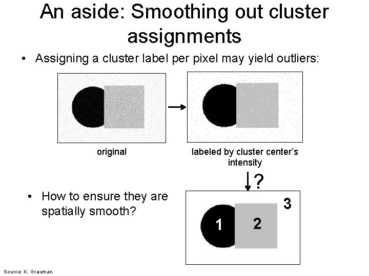
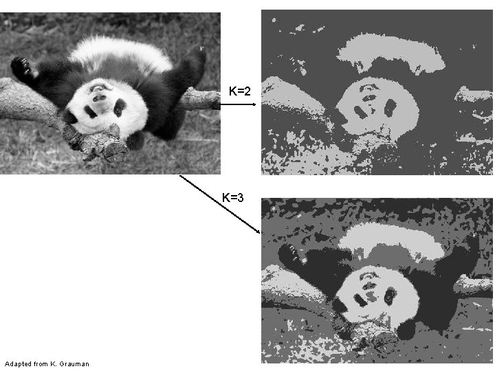
An aside: Smoothing out cluster assignments • Assigning a cluster label per pixel may yield outliers: original • How to ensure they are spatially smooth? Source: K. Grauman labeled by cluster center’s intensity ? 3 1 2

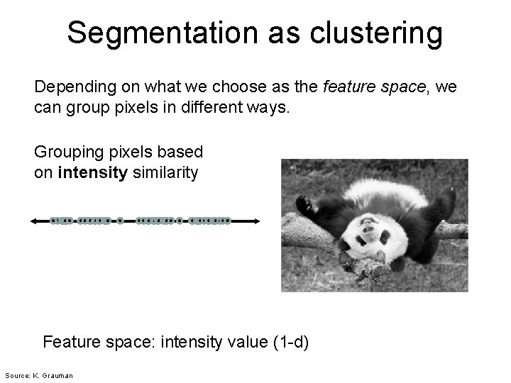
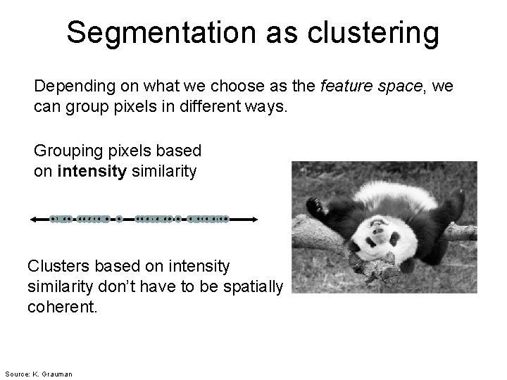
Segmentation as clustering Depending on what we choose as the feature space, we can group pixels in different ways. Grouping pixels based on intensity similarity Feature space: intensity value (1 -d) Source: K. Grauman

K=2 K=3 Adapted from K. Grauman

Segmentation as clustering Depending on what we choose as the feature space, we can group pixels in different ways. Grouping pixels based on intensity similarity Clusters based on intensity similarity don’t have to be spatially coherent. Source: K. Grauman

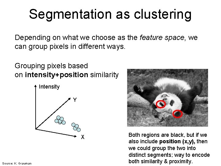
Segmentation as clustering Depending on what we choose as the feature space, we can group pixels in different ways. Grouping pixels based on intensity+position similarity Intensity Y X Source: K. Grauman Both regions are black, but if we also include position (x, y), then we could group the two into distinct segments; way to encode both similarity & proximity.

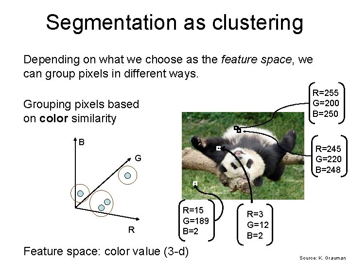
Segmentation as clustering Depending on what we choose as the feature space, we can group pixels in different ways. R=255 G=200 B=250 Grouping pixels based on color similarity B R=245 G=220 B=248 G R R=15 G=189 B=2 Feature space: color value (3 -d) R=3 G=12 B=2 Source: K. Grauman

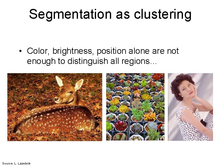
Segmentation as clustering • Color, brightness, position alone are not enough to distinguish all regions… Source: L. Lazebnik

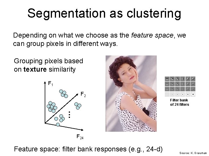
Segmentation as clustering Depending on what we choose as the feature space, we can group pixels in different ways. Grouping pixels based on texture similarity F 1 F 2 Filter bank of 24 filters … F 24 Feature space: filter bank responses (e. g. , 24 -d) Source: K. Grauman

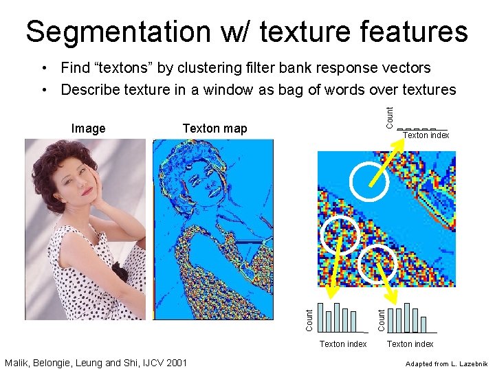
Segmentation w/ texture features Texton map Count Texton index Count Image Count • Find “textons” by clustering filter bank response vectors • Describe texture in a window as bag of words over textures Texton index Malik, Belongie, Leung and Shi, IJCV 2001 Texton index Adapted from L. Lazebnik

Summary • Edges: threshold gradient magnitude • Lines: edge points vote for parameters of line, circle, etc. (works for general objects) • Segments: use clustering (e. g. K-means) to group pixels by intensity, texture, etc.