Cosmic Rays in the Heliosphere J R Jokipii


 and galactic cosmic rays (GCR).")

 Diffusion ) Convection w. plasma ) Grad & Curvature")


 reports significant anisotropies. The anisotropy is ~ few % and persists")

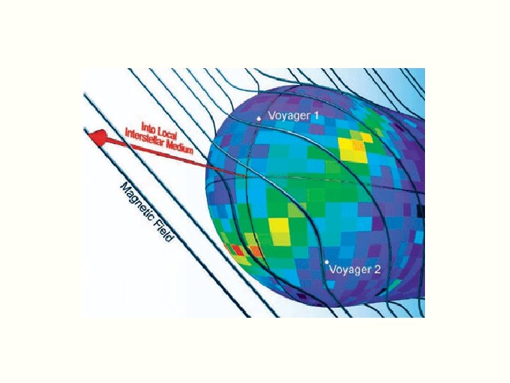
 Note the decrease in |B| near the heliopause. This is the result of")


- Slides: 27
Cosmic Rays in the Heliosphere J. R. Jokipii University of Arizona I acknowledge helpful discussions with J. Kόta and J. GIacalone. Presented at the Te. V Particle Astrophysics Workshop, Irvine, CA, 26 -29 August, 2013
Cosmic Rays Helio s Effec pheric ts
• I will concentrate on energies significantly lower than 1 Te. V, as the effects of the heliosphere at 1 Te. V are smaller (but still significant). • The gyro-radius of a 1 Te. V proton in the interstellar magnetic field is ~ 74 AU, which is signifiantly smaller than the heliosphere. • The interstellar field is distorted in the flow around the heliosphere out to perhaps a few hundred AU, so there should be significant observable effects on cosmic rays up to 10 Te. V or more. • I do not have time to discuss this further here.
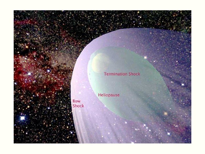
The standard paradigm for anomalous cosmic rays (ACR) and galactic cosmic rays (GCR).
Solar Particles Showing the average GCR intensity at Earth with very transient solar particles superimposed. A solar energetic-particle event lasts hours to a day or so. The average intensity at energies > 100 Me. V/nuc is dominated by GCRs and anomalous cosmic rays. Until the past year, we had no knowledge of the GCR flux below some 100 Me. V/nuc. galactic
The Parker Transport Equation: ) Diffusion ) Convection w. plasma ) Grad & Curvature Drift ) Energy change ) Source Where the drift velocity due to the large scale curvature and gradient of the average magnetic field is:
Let us look at the paradigm of diffusive shock acceleration for a simple planar shock. Solve Parker’s equation at a flow discontinuity.
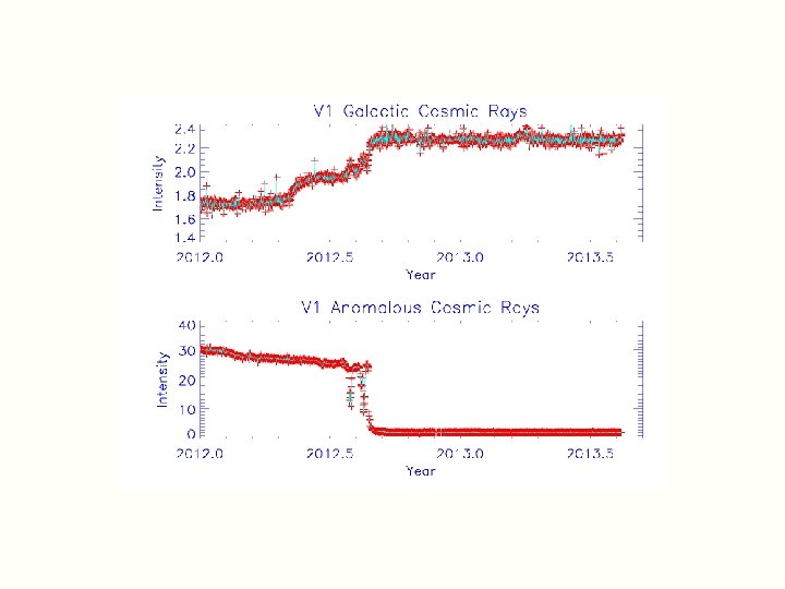
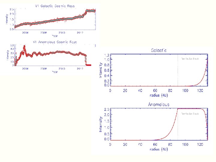
We believe that V 1 is now observing the interstellar GCR intensity below 200 Me. V for the very first time!
What is the interpretation of these recent changes in the energetic particles? • Given the general agreement with the expected behavior at the heliopase, the observations prompted speculation that the heliopause was indeed crossed. • The magnetometer data was eagerly anticipated. It was expected that the magnetic field would show a change in direction at the same time as the intensity changes in ACR and GCR.
However, the V 1 magnetometer showed no significant change in direction. Hence, the Voyager SSG has decided that this is a new region of space – the ‘magnetic highway’. ) Some feel that V 1 crossed the heliopause and others that V 1 has not. This is currently being debated.
Galactic cosmic rays have been observed in many observations over the last several decades to be very nearly isotropic. At several Te. V energies, the -3 anisotropies observed are less than 10. At lower energies, one must use modeling, as the heliosphere distorts the trajectories of the lowerenergy particles. This analysis has been done by many authors.
Pohl and Eichler 2013 Ap. J 766 4 doi: 10. 1088/0004 -637 X/766/1/4 Extrapolating to ~Ge. V energies yields a very small anisotropy ~10 -4
Hill (private communication) reports significant anisotropies. The anisotropy is ~ few % and persists for several months. This is the larges GCR anisotropy ever observed.
What can be the cause of this large anisotropy? Almost certainly it is not of interstellar origin. It must come from the interaction of the interstellar medium with the heliosphere.
) Note the decrease in |B| near the heliopause. This is the result of a simulation sent to me by M. Opher. (Pogorelov shows similar curves. )
Effects of variation in the magnetic-field intensity on isotropy • We consider 200 Me. V galactic cosmic rays. • Their gyroradius in the 3 n. T local interstellar magnetic field is rg = m w c/(q B)=. 033 AU and their gyro-period is ¿g = 2 ¼/!g = 125 sec. • The corresponding scales in the local ISM flow around the heliopause are L ¼ AU, and ¿flow = L/Uflow ¼ 2. 5 yr. • Hence, on scales less than the scattering mean free path, the cosmic-ray motion conserves the first adiabatic invariant ¹ad = Tperp / B, where Tperp is the perpendicular kinetic energy. • Changes in the magnetic field magnitude B will therefore induce anisotropies in an originally isotropic distribution, unless scattering by the turbulence isotropizes the distribution faster, on a shorter time scale.
Similar to observation
Effect of scattering. • Interstellar turbulence scatters the cosmic rays. • The time scale for this may be estimated from the interstellar diffusion coefficient deduced from a number of different observations. • One finds ·ism ¼ 1027 -1028 cm 2/sec for 200 Me. V protons. • In this case, ¸sc ¼ 1. 5 x 1018 cm or ¿sc ¼ 2. 5 yr. • Thus the scattering time and the flow time scale are comparable, so scattering plays a role. • We expect some anisotropy, but not as much as that given by adiabatic invariant conservation. • We must carry out a numerical analysis.
Solve for the distribution function • Use Liouville’s equation. • Apply to an initially isotropic distribution with a dependence on momentum given by f 0(p) = Ap-° with ° = -2. 6. • Scattering is taken to be simple isotropization with a scattering time ¿sc. • The magnetic field decreases or increases, causing an anisotropy. Scattering counters this.
Solution for a magnetic field decreasing to 0. 7 of its original value, with various values of ¿sc approximately that of interstellar scattering. The magnitude of the anisotropy is not far from what is observed.
Solution for a magnetic field decreasing to 0. 9 of its original value, with various values of ¿sc.
Effect of an increasing magnetic field. This is not what is observed.
Conclusions • The effects of the flow of the around the heliosphere on cosmic rays and the consequent change in magnetic-field magnitude produces either bi-directional field-alligned or pancake anisotropies. • Whether the anisotropy is field-aligned or pancake depends on whether the field increases or decreases. • These anisotropies are consistent with recent preliminary observations of ~ 200 Me. V galactic cosmic rays. • Further analysis should provide valuable information concerning the transport of galactic cosmic rays.