Chapters 8 9 10 Least Squares Regression Line

Chapters 8, 9, 10 Least Squares Regression Line Fitting a Line to Bivariate Data

Suppose there is a relationship between two numerical variables. Data: (x 1, y 1), (x 2, y 2), …, (xn, yn) Let x be the amount spent on advertising and y be the amount of sales for the product during a given le b a i r a v e period. h noted t de o t d e e s s u n o s i p s y e r r e h t d e l he lette l T a c , t c i d e r You might want to predict product sales for a p o t t n a ou w y monthab(y) when the amount spent on advertizing. e l i v. Tahre ot is $10, 000 her(x). variable, denoted explanat by x, is t ory varia he ble.

Simplest Relationship • Simplest equation that describes the dependence of variable y on variable x y = b 0 + b 1 x • linear equation • b 1 is the slope – it is the amount by which y changes when x increases by 1 unit • y-intercept b 0 – where the line crosses the y-axis; that is, the value of y when x = 0.

Graph is a line y=b 0 +b 1 x y rise b 0 Slope b=rise/run 0 x

How do you find an appropriate line for Let’s look at only the blue line. describing a bivariate data set? The point (15, 44) has a deviation To assess fitaof a line, we a To assess the fit of line, we need at how the n points deviate way look to combine deviations into a vertically from the line. single measure of fit. of +4. y = 4 + 2. 5 x What is the meaning of a negative deviation? y = 10 + 2 x

The deviations are referred to as residuals and denoted ei.

Residuals: graphically

The Least Squares (Regression) Line A good line is one that minimizes the sum of squared differences between t points and the line. 8

The Least Squares (Regression) Line Sum of squared differences (2 - =1)2 + (4 - 2)2 (+1. 5 - 3)2 + (3. 2 - 4)2 = 6. 89 Sum of squared differences (2 -2. 5) = 2+ (4 - 2. 5)2 (+1. 5 - 2. 5)2 (3. 2 + - 2. 5)2 = 3. 99 3 2. 5 2 Let us compare two lines The second line is horizonta (2, 4) w 4 w (4, 3. 2) (1, 2)w w (3, 1. 5) 1 1 2 3 4 The smaller the sum of squared differences the better the fit of the line to the data. 9

Criterion for choosing what line to draw: method of least squares • The method of least squares chooses the line that makes the sum of squares of the residuals as small as possible • This line has slope b 1 and intercept b 0 that minimizes

Least Squares Line y = b 0 + b 1 x: Slope b 1 and Intercept b 0

Scatterplot with least squares prediction line (xi, yi): (3. 4, 5. 5) (3. 8, 5. 9) (4. 1, 6. 5) (2. 2, 3. 3) (2. 6, 3. 6) (2. 9, 4. 6) (2, 2. 9) (2. 7, 3. 6) (1. 9, 3. 1) (3. 4, 4. 9)

Observed y, Predicted y FUEL CONSUMPTION vs CAR WEIGHT 7 6, 5 6 5, 5 5 4, 5 4 3, 5 3 2, 5 2 predicted y when x=2. 7 = b 0 + b 1 x = b 0 + b 1*2. 7 (2. 7, 3. 6) 3. 6 = observed y 1, 5 2 2, 5 2. 7 3 CAR WEIGHT 3, 5 4 4, 5

Car Weight, Fuel Consumption Example, cont. (xi, yi): (3. 4, 5. 5) (3. 8, 5. 9) (4. 1, 6. 5) (2. 2, 3. 3) (2. 6, 3. 6) (2. 9, 4. 6) (2, 2. 9) (2. 7, 3. 6) (1. 9, 3. 1) (3. 4, 4. 9)

col. sum Wt (x) Fuel (y) 3. 4 5. 5 . 25 1. 11 1. 231 3. 8 5. 9 . 81 1. 51 2. 2801 1. 359 4. 1 6. 5 1. 2 1. 44 2. 11 4. 4521 2. 532 2. 2 3. 3 -. 7 . 49 -1. 09 1. 1881. 763 2. 6 3. 6 -. 3 . 09 -. 79 . 6241 . 237 2. 9 4. 6 0 0 . 21 . 0441 0 2. 9 -. 9 . 81 -1. 49 2. 2201 1. 341 2. 7 3. 6 -. 2 . 04 -. 79 1. 9 3. 1 -1. 0 1 -1. 29 1. 6641 1. 29 3. 4 4. 9 . 5 . 25 . 51 . 2601 29 43. 9 0 5. 18 0 14. 589 8. 49 . 6241 . 555 . 158 . 255

Calculations

Scatterplot with least squares prediction line

FUEL CONSUMP. (gal/100 miles) The Least Squares Line Always goes Through ( x, y ) FUEL CONSUMPTION vs CAR WEIGHT 7 6, 5 6 5, 5 5 4, 5 4 3, 5 3 2, 5 2 (x, y ) = (2. 9, 4. 39) 1, 5 2, 5 WEIGHT (1000 lbs) 3, 5 4, 5

Using the least squares line for prediction. Fuel consumption of 3, 000 lb car? (x=3)

Be Careful! Fuel consumption of 500 lb car? (x =. 5) x =. 5 is outside the range of the x-data that we used to determine the least squares line

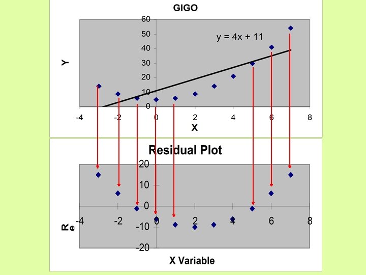
Avoid GIGO! Evaluating the least squares line 1. Create scatterplot. Approximately linear? 2. Calculate r 2, the square of the correlation coefficient 3. Examine residual plot

r 2 : The Variation Accounted For • The square of the correlation coefficient r gives important information about the usefulness of the least squares line

r 2: important information for evaluating the usefulness of the least squares line -1 ≤ r ≤ 1 implies 0 ≤ r 2 ≤ 1 The square of the correlation coefficient, r 2, is the fraction of the variation in y that is explained by the least squares regression of y on x. The square of the correlation coefficient, r 2, is the fraction of the variation in y that is explained by differences in x.

March Madness: S(k) Sagarin rating of kth seeded team; Yij =Vegas point spread between seed i and seed j, i<jof the variation in point 94. 8% spreads is explained by the variation in Sagarin ratings.

SAT scores: result r 2 = (-. 86845)2 =. 7542 Approx. 75. 4% of the variation in mean SAT math scores is explained by differences in the percent of seniors taking the SAT.

Avoid GIGO! Evaluating the least squares line 1. Create scatterplot. Approximately linear? 2. Calculate r 2, the square of the correlation coefficient 3. Examine residual plot

Residuals • residual • Properties of residuals =observed y - predicted y = y y 1. The residuals always sum to 0 (therefore the mean of the residuals is 0) 2. The least squares line always goes through the point (x, y)

y Graphically residual = y - y yi yi ei=yi - yi X xi

Residual plots • A residual plot is a scatterplot of the careful look at the residuals can residual)Apairs. reveal many potential problems. (x, • Residuals. Acan also beplot graphed against the residual is a graph of the predicted y-values residuals. • We make a scatterplot of the residuals in the hope of finding…NOTHING! • Isolated points or a pattern of points in the residual plot indicate potential problems.

Car weight, fuel consumption, continued Weight(x) Fuel Consumption (y) Predicted Fuel Consump. Residual 3. 4 5. 5 5. 21 0. 29 3. 8 5. 9 5. 87 0. 03 4. 1 6. 5 6. 36 0. 14 2. 2 3. 3 3. 24 0. 06 2. 6 3. 90 -0. 30 2. 9 4. 6 4. 39 0. 21 2. 0 2. 91 -0. 01 2. 7 3. 6 4. 06 -0. 46 1. 9 3. 1 2. 75 0. 35 3. 4 4. 9 5. 21 -0. 31 Plot the residuals against the Weight (x)

Weight(x) Residual 3. 4 0. 29 3. 8 0. 03 4. 1 0. 14 2. 2 0. 06 2. 6 -0. 30 2. 9 0. 21 2. 0 -0. 01 2. 7 -0. 46 1. 9 0. 35 3. 4 -0. 31

Residuals: Sagarin Ratings and Point Spreads Yij 20 24 18 11 6 8. 5 4 4 28 16 11. 5 12 4 7 -1. 5 2 Predicted Yij 23. 48573586 21. 3717734 13. 96719139 11. 52185104 5. 774158519 7. 613877198 1. 683355495 2. 186135755 27. 26801463 15. 53266629 10. 56199781 10. 11635167 5. 397073324 6. 836853159 1. 500526309 1. 946172449 Residuals -3. 485735859 2. 628226598 4. 032808608 -0. 521851036 0. 225841481 0. 886122802 2. 316644505 1. 813864245 0. 731985367 0. 467333708 0. 938002187 1. 883648327 -1. 397073324 0. 163146841 -3. 000526309 0. 053827551 Yij 25 18. 5 10. 5 11. 5 4. 5 5 4 -3. 5 23 20. 5 18 10. 5 9 7 2 5 Predicted Yij 23. 58857728 18. 34366502 12. 85878945 10. 95050983 2. 597501422 6. 631170326 3. 203123099 0. 095026946 24. 15991848 21. 24607834 20. 0919691 11. 62469245 6. 836853159 5. 979841353 3. 283110867 6. 745438567 Residuals 1. 411422725 0. 156334982 -2. 358789455 0. 549490168 1. 902498578 -1. 631170326 0. 796876901 -3. 595026946 -1. 15991848 -0. 746078337 -2. 091969104 -1. 124692453 2. 163146841 1. 020158647 -1. 283110867 -1. 745438567

Plot of Sagarin Residuals Good!

Linear Relationship?

Garbage In Garbage Out

Residual Plot – Clue to GIGO