Chapter 2 Introduction to Optimization and Linear Programming

Chapter 2 Introduction to Optimization and Linear Programming (LP)

Introduction § We all face decisions about how to use limited resources such as: – Machines – Land – Time – Money – Workers

Mathematical Programming. . . § Mathematical Programming is a field of management science that finds the optimal or best way of using limited resources to achieve the objectives of a business. § a. k. a. Optimization. In this course we will use a powerful tool called Linear Programming (LP) to help us find the best (i. e. , optimal) solutions.

Applications of Optimization § § Determining Product Mix Manufacturing Logistics Financial Planning

Characteristics of Optimization Problems § Decisions Variables (e. g. , what is unknown). § Constraints (e. g. , limited availability of money, employees, or machines) § Objectives (e. g. , maximize profit or minimize cost). How about some examples!

Example 1: Determining Product Mix A manager needs to know how many TV’s, VCR’s, and Radios to produce in the next production period to maximize total profit. Decision variables: how many TV’s, VCR’s, and Radios to produce. Constraints: manager has a limited budget, number of employees and machines. Objective: Maximize profit.

Example 2: Logistics Assume that Wal-Mart has 10 distribution centers and 50 retail stores in the state of Pennsylvania. Every retail outlet has a given demand for a given product that must be met. Also, every distribution center has a limited supply quantity of each product. We want to determine the optimal shipping strategy that will minimize total shipping cost. What are the decision variables, constraints, and objective function? See next slide for the solution!

Example 2 Solution Decision Variables: How many units of each product to ship from each distribution center to each retail outlet. Constraints: We’ll have 2 sets of constraints. Set 1 will ensure that each distribution center does not ship more that its capacity (i. e. , supply constraints), while set 2 will ensure that the demand requirements of each retail outlet is satisfied (i. e. , demand constraints). Objective: Minimize total shipping cost.

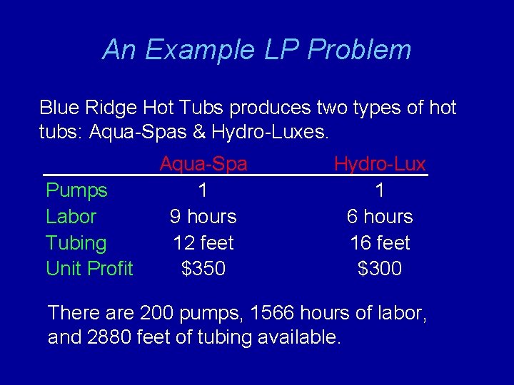
An Example LP Problem Blue Ridge Hot Tubs produces two types of hot tubs: Aqua-Spas & Hydro-Luxes. Pumps Labor Tubing Unit Profit Aqua-Spa 1 9 hours 12 feet $350 Hydro-Lux 1 6 hours 16 feet $300 There are 200 pumps, 1566 hours of labor, and 2880 feet of tubing available.

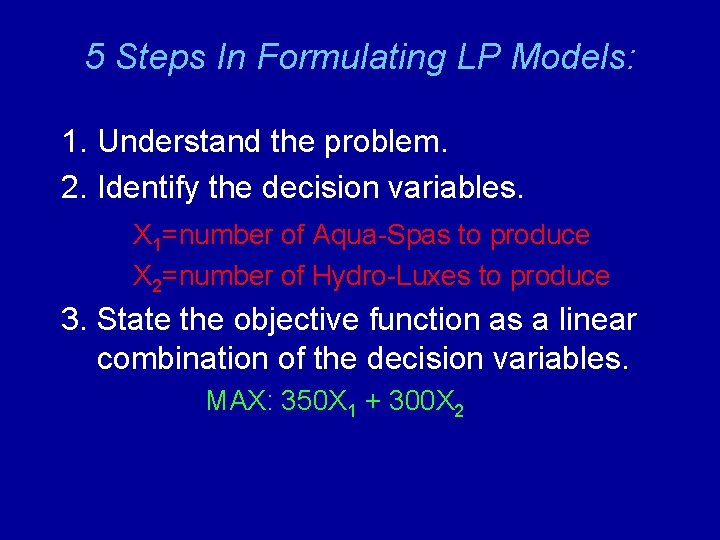
5 Steps In Formulating LP Models: 1. Understand the problem. 2. Identify the decision variables. X 1=number of Aqua-Spas to produce X 2=number of Hydro-Luxes to produce 3. State the objective function as a linear combination of the decision variables. MAX: 350 X 1 + 300 X 2

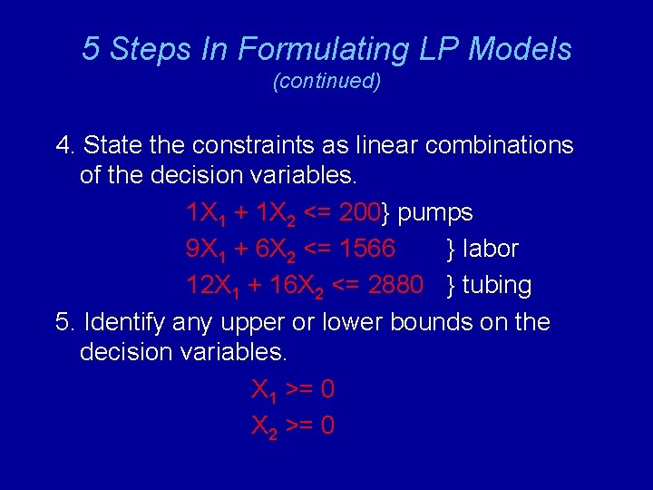
5 Steps In Formulating LP Models (continued) 4. State the constraints as linear combinations of the decision variables. 1 X 1 + 1 X 2 <= 200} pumps 9 X 1 + 6 X 2 <= 1566 } labor 12 X 1 + 16 X 2 <= 2880 } tubing 5. Identify any upper or lower bounds on the decision variables. X 1 >= 0 X 2 >= 0

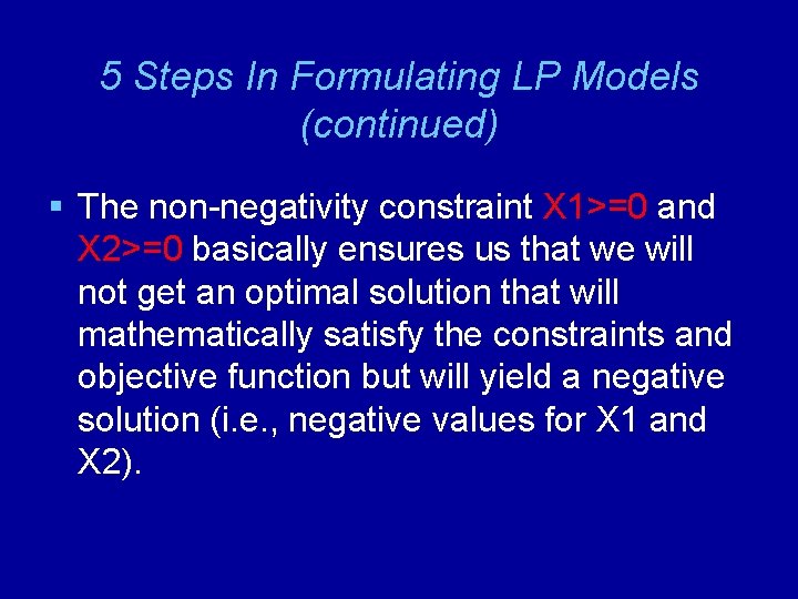
5 Steps In Formulating LP Models (continued) § The non-negativity constraint X 1>=0 and X 2>=0 basically ensures us that we will not get an optimal solution that will mathematically satisfy the constraints and objective function but will yield a negative solution (i. e. , negative values for X 1 and X 2).

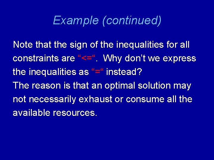
Example (continued) Note that the sign of the inequalities for all constraints are “<=“. Why don’t we express the inequalities as “=“ instead? The reason is that an optimal solution may not necessarily exhaust or consume all the available resources.

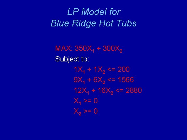
LP Model for Blue Ridge Hot Tubs MAX: 350 X 1 + 300 X 2 Subject to: 1 X 1 + 1 X 2 <= 200 9 X 1 + 6 X 2 <= 1566 12 X 1 + 16 X 2 <= 2880 X 1 >= 0 X 2 >= 0

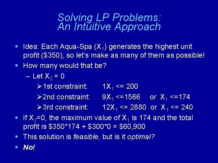
Solving LP Problems: An Intuitive Approach § Idea: Each Aqua-Spa (X 1) generates the highest unit profit ($350), so let’s make as many of them as possible! § How many would that be? – Let X 2 = 0 Ø 1 st constraint: 1 X 1 <= 200 Ø 2 nd constraint: 9 X 1 <=1566 or X 1 <=174 Ø 3 rd constraint: 12 X 1 <= 2880 or X 1 <= 240 § If X 2=0, the maximum value of X 1 is 174 and the total profit is $350*174 + $300*0 = $60, 900 § This solution is feasible, but is it optimal? § No!

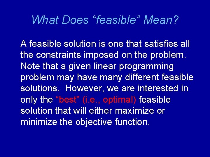
What Does “feasible” Mean? A feasible solution is one that satisfies all the constraints imposed on the problem. Note that a given linear programming problem may have many different feasible solutions. However, we are interested in only the “best” (i. e. , optimal) feasible solution that will either maximize or minimize the objective function.

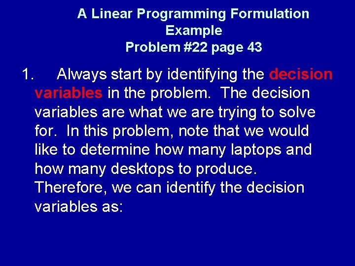
A Linear Programming Formulation Example Problem #22 page 43 1. Always start by identifying the decision variables in the problem. The decision variables are what we are trying to solve for. In this problem, note that we would like to determine how many laptops and how many desktops to produce. Therefore, we can identify the decision variables as:

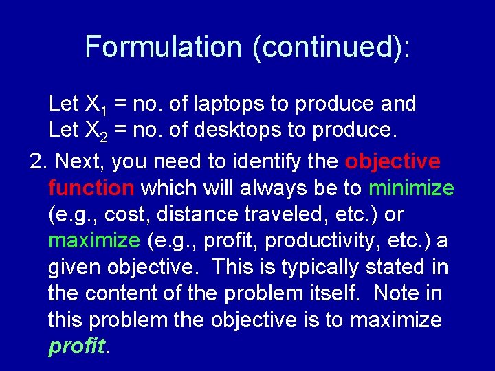
Formulation (continued): Let X 1 = no. of laptops to produce and Let X 2 = no. of desktops to produce. 2. Next, you need to identify the objective function which will always be to minimize (e. g. , cost, distance traveled, etc. ) or maximize (e. g. , profit, productivity, etc. ) a given objective. This is typically stated in the content of the problem itself. Note in this problem the objective is to maximize profit.

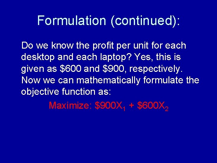
Formulation (continued): Do we know the profit per unit for each desktop and each laptop? Yes, this is given as $600 and $900, respectively. Now we can mathematically formulate the objective function as: Maximize: $900 X 1 + $600 X 2

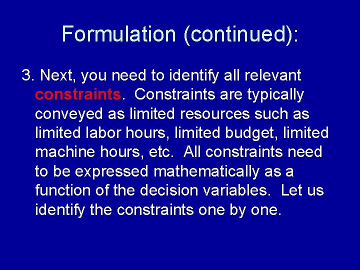
Formulation (continued): 3. Next, you need to identify all relevant constraints. Constraints are typically conveyed as limited resources such as limited labor hours, limited budget, limited machine hours, etc. All constraints need to be expressed mathematically as a function of the decision variables. Let us identify the constraints one by one.

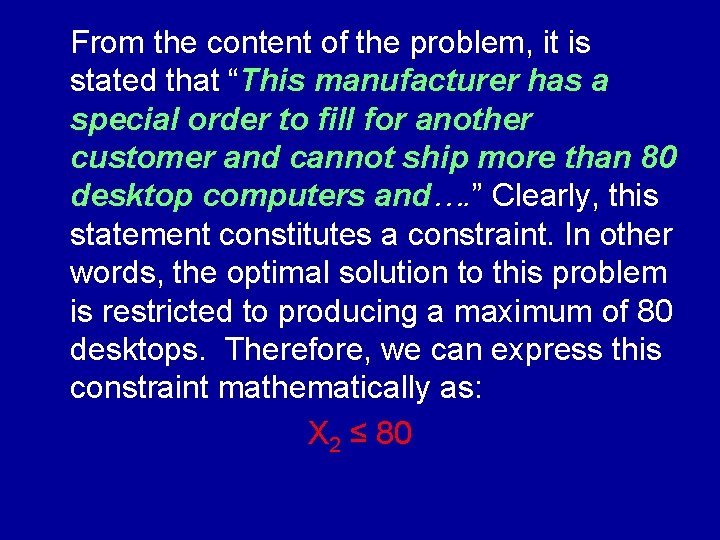
From the content of the problem, it is stated that “This manufacturer has a special order to fill for another customer and cannot ship more than 80 desktop computers and…. ” Clearly, this statement constitutes a constraint. In other words, the optimal solution to this problem is restricted to producing a maximum of 80 desktops. Therefore, we can express this constraint mathematically as: X 2 ≤ 80

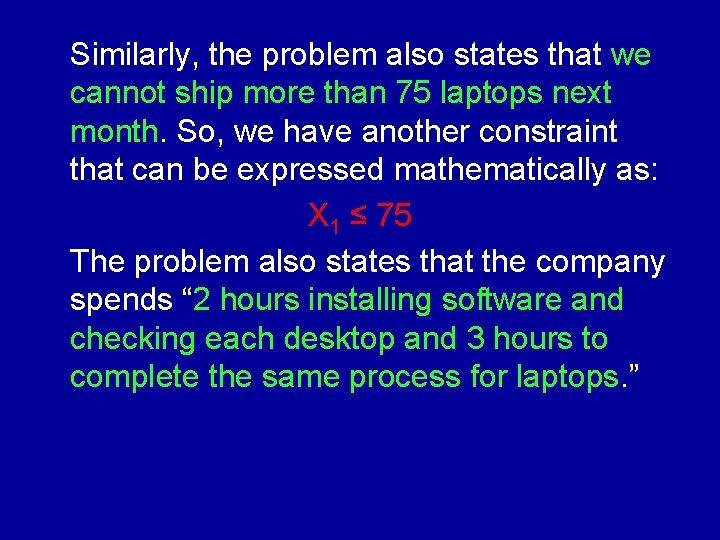
Similarly, the problem also states that we cannot ship more than 75 laptops next month. So, we have another constraint that can be expressed mathematically as: X 1 ≤ 75 The problem also states that the company spends “ 2 hours installing software and checking each desktop and 3 hours to complete the same process for laptops. ”

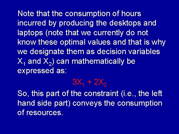
Note that the consumption of hours incurred by producing the desktops and laptops (note that we currently do not know these optimal values and that is why we designate them as decision variables X 1 and X 2) can mathematically be expressed as: 3 X 1 + 2 X 2 So, this part of the constraint (i. e. , the left hand side part) conveys the consumption of resources.

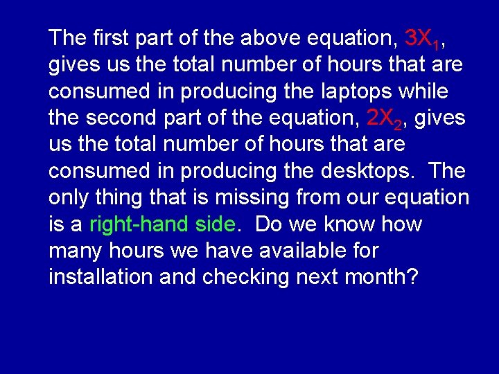
The first part of the above equation, 3 X 1, gives us the total number of hours that are consumed in producing the laptops while the second part of the equation, 2 X 2, gives us the total number of hours that are consumed in producing the desktops. The only thing that is missing from our equation is a right-hand side. Do we know how many hours we have available for installation and checking next month?

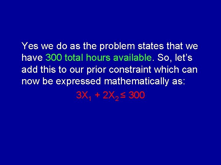
Yes we do as the problem states that we have 300 total hours available. So, let’s add this to our prior constraint which can now be expressed mathematically as: 3 X 1 + 2 X 2 ≤ 300

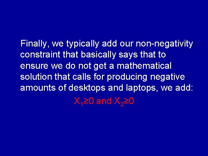
Finally, we typically add our non-negativity constraint that basically says that to ensure we do not get a mathematical solution that calls for producing negative amounts of desktops and laptops, we add: X 1≥ 0 and X 2≥ 0

Solving LP Problems: A Graphical Approach § The constraints of an LP problem defines its feasible region. § The best point in the feasible region is the optimal solution to the problem. § For LP problems with 2 variables, it is easy to plot the feasible region and find the optimal solution.

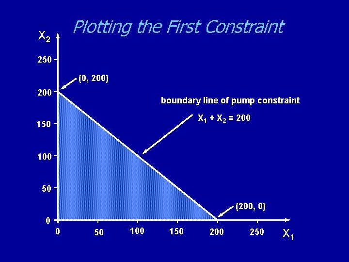
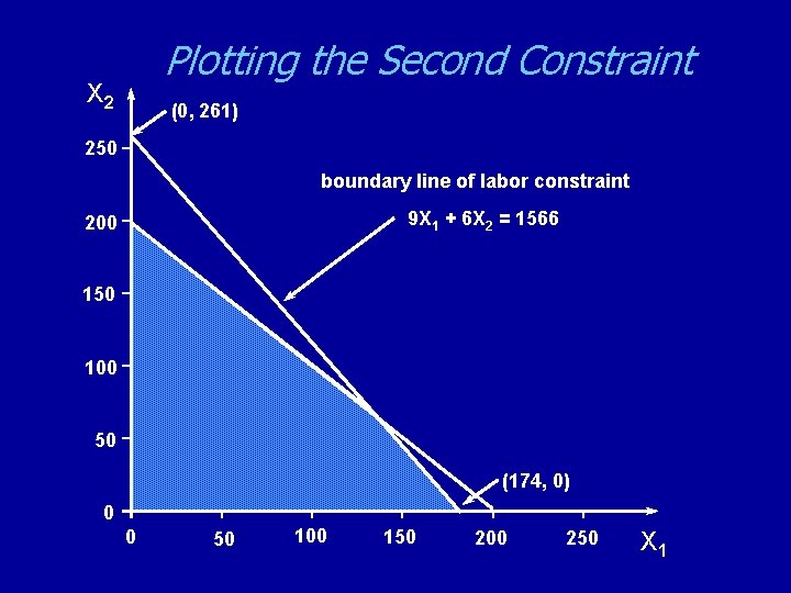
Guidelines on Plotting Constraints All constraints are represented as straight lines as long as they are linear in nature. So, first ignore the sign of the inequality and replace it with an equality “=“ sign. Next, to find where a constraint intercepts the X 1 axis, plug X 1=0 and solve for X 2. This will give us the coordinates (0, X 2) Now to find where the constraint intercepts the X 2 axis, plug X 2=0 and solve for X 1. This will give us the coordinates of the second point (X 1, 0)

Plotting Constraints Guidelines (continued) Now you have 2 points that the straight line equation goes through, so connect the 2 points. Finally, let’s put back the original inequality sign. In general, “<=“ constraints span a region that points toward the origin (i. e. , coordinates (0, 0)). Also, in general, “>=“ constraints span a region that points in the opposite direction of the origin. This notion is explained in more detail in the two animated videos that you will be watching shortly.

Summary of Graphical Solution to LP Problems 1. Plot the boundary line of each constraint 2. Identify the feasible region 3. Locate the optimal solution by using either: a. The level curves, or b. The corner points approach

Plotting the First Constraint X 2 250 (0, 200) 200 boundary line of pump constraint X 1 + X 2 = 200 150 100 50 (200, 0) 0 0 50 100 150 200 250 X 1

Plotting the Second Constraint X 2 (0, 261) 250 boundary line of labor constraint 9 X 1 + 6 X 2 = 1566 200 150 100 50 (174, 0) 0 0 50 100 150 200 250 X 1

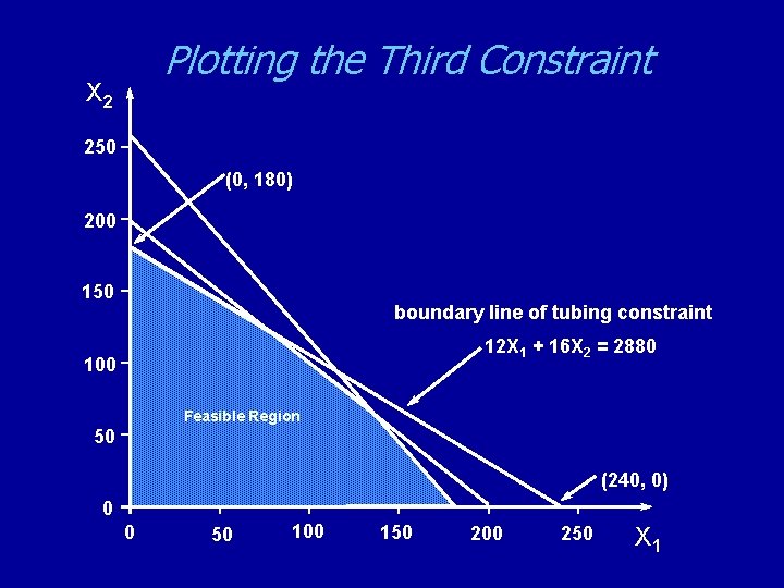
Plotting the Third Constraint X 2 250 (0, 180) 200 150 boundary line of tubing constraint 12 X 1 + 16 X 2 = 2880 100 Feasible Region 50 (240, 0) 0 0 50 100 150 200 250 X 1

Some Thoughts Note that the feasible region is the shaded area that is dictated by the constraints. Any point inside this feasible region is a possible solution to the problem. However, note that there are thousands or perhaps millions of feasible solutions. So, how do we pinpoint the optimal solution?

Determining the Optimal Solution In general, there are 2 methods that can be employed to find the optimal solution: 1. The Level Curves approach. 2. The Corner-Point enumeration.

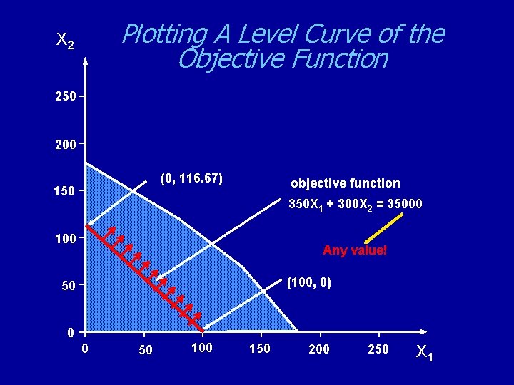
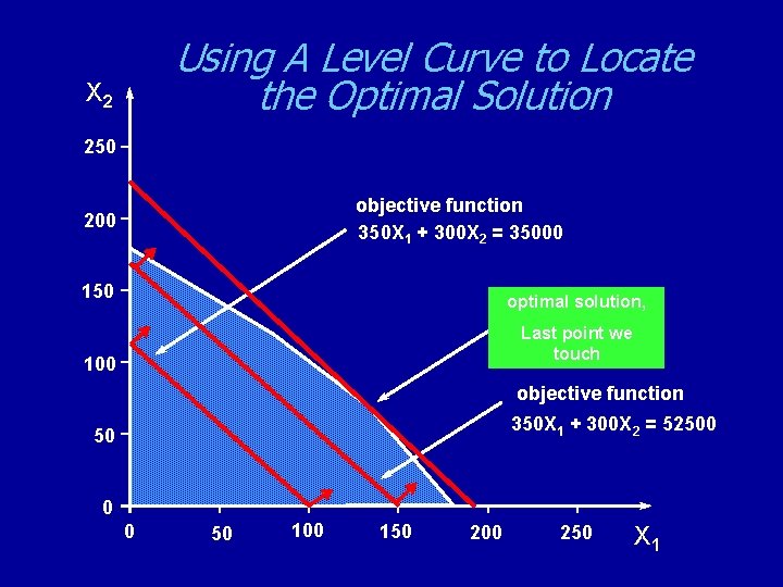
Level Curves Approach Assume any value for the objective function. Next, plot this straight line equation on the same graph where you identified the feasible region. Using a straight edge, move this line (keeping it parallel, upward if maximizing and downward if minimizing) until you hit/touch the last point of the feasible region. This point will be your optimal solution!

Level Curves (continued) But how do you determine the coordinates of this optimal point? In general, you will have to solve simultaneously the two equations, that is the two constraints, that formed this point. Also, note that in general, the optimal solution occurs at a corner point.

Corner Point Enumeration In general the optimal solution will lie at a corner point of the feasible region. So, this method will identify the coordinates of each corner point. Plug each coordinate point into the objective function. If the objective function is maximization, then you are looking for the corner point with the highest value. If the objective function is minimization, you are looking for the corner point that will minimize the objective function.

Which Method is Better? The level curves approach is more efficient because you will typically solve for only one set of simultaneous equations rather than many. However, regardless of the approach used, both methods will yield identical results. Now let’s go back to the Hot Tubs example!

Plotting A Level Curve of the Objective Function X 2 250 200 (0, 116. 67) 150 objective function 350 X 1 + 300 X 2 = 35000 100 Any value! (100, 0) 50 0 0 50 100 150 200 250 X 1

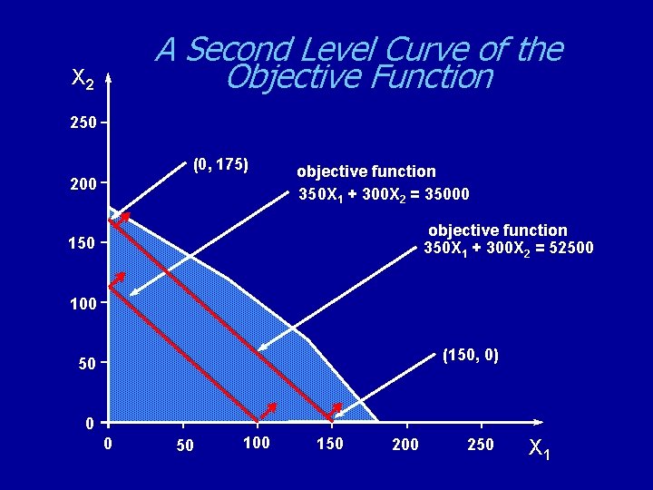
A Second Level Curve of the Objective Function X 2 250 (0, 175) 200 objective function 350 X 1 + 300 X 2 = 35000 objective function 350 X 1 + 300 X 2 = 52500 150 100 (150, 0) 50 0 0 50 100 150 200 250 X 1

Using A Level Curve to Locate the Optimal Solution X 2 250 objective function 350 X 1 + 300 X 2 = 35000 200 150 optimal solution, Last point we touch 100 objective function 350 X 1 + 300 X 2 = 52500 50 0 0 50 100 150 200 250 X 1

Level Curves Method So, let’s recap what we have done so far. First we assumed any value for the objective function which is 35000. Next we plotted this line (i. e. , 350 X 1 + 300 X 2 = 35000). Now, since the objective function is a maximization one, we would like to push this line that we have just plotted upward until we touch the last corner point of the feasible region. This last point will be the optimal point.

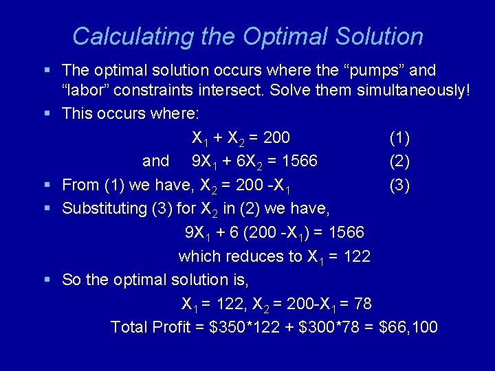
Calculating the Optimal Solution § The optimal solution occurs where the “pumps” and “labor” constraints intersect. Solve them simultaneously! § This occurs where: X 1 + X 2 = 200 (1) and 9 X 1 + 6 X 2 = 1566 (2) § From (1) we have, X 2 = 200 -X 1 (3) § Substituting (3) for X 2 in (2) we have, 9 X 1 + 6 (200 -X 1) = 1566 which reduces to X 1 = 122 § So the optimal solution is, X 1 = 122, X 2 = 200 -X 1 = 78 Total Profit = $350*122 + $300*78 = $66, 100

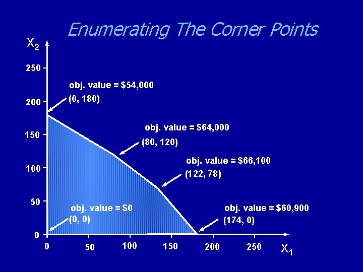
Corner Point Method This method is quite simple. Compute the coordinates of all the corner points of the feasible region. Next, plug the coordinates of each corner point into the objective function. Since our problem is a maximization one, the corner point with the highest objective function value will be the optimal solution.

Enumerating The Corner Points X 2 250 obj. value = $54, 000 (0, 180) 200 obj. value = $64, 000 150 (80, 120) obj. value = $66, 100 (122, 78) 100 50 obj. value = $60, 900 (174, 0) obj. value = $0 (0, 0) 0 0 50 100 150 200 250 X 1

Enumerating The Corner Points § Once again, how do we know in the prior slide the coordinates for each corner point? If you recall we need to solve simultaneously for the two constraints (i. e. , the two straight lines) that formed each corner.

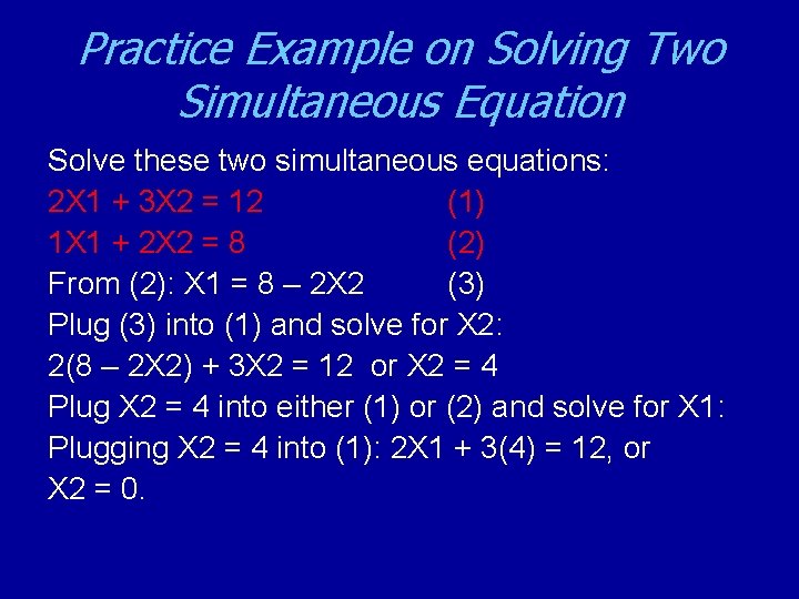
Practice Example on Solving Two Simultaneous Equation Solve these two simultaneous equations: 2 X 1 + 3 X 2 = 12 (1) 1 X 1 + 2 X 2 = 8 (2) From (2): X 1 = 8 – 2 X 2 (3) Plug (3) into (1) and solve for X 2: 2(8 – 2 X 2) + 3 X 2 = 12 or X 2 = 4 Plug X 2 = 4 into either (1) or (2) and solve for X 1: Plugging X 2 = 4 into (1): 2 X 1 + 3(4) = 12, or X 2 = 0.

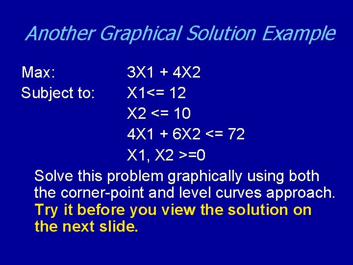
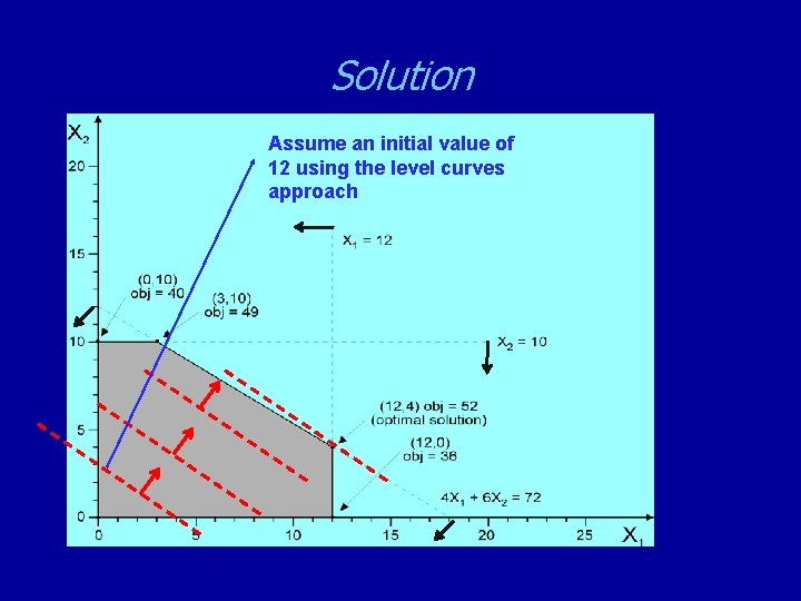
Another Graphical Solution Example Max: Subject to: 3 X 1 + 4 X 2 X 1<= 12 X 2 <= 10 4 X 1 + 6 X 2 <= 72 X 1, X 2 >=0 Solve this problem graphically using both the corner-point and level curves approach. Try it before you view the solution on the next slide.

Solution Assume an initial value of 12 using the level curves approach

Graphical Solution Method Video Clips § Now will be a good time to view the two video clips that I have prepared for you in order to enhance/aid your understanding of the graphical solution method, so please view them from Week 1 Multimedia, under the heading Animation.

Special Conditions in LP Models § A number of “anomalies” can occur in LP problems where we will just refer to them as “Special Cases”: – Alternate Optimal Solutions – Redundant Constraints – Unbounded Solutions – Infeasibility

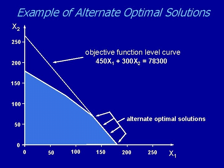
Example of Alternate Optimal Solutions X 2 250 objective function level curve 450 X 1 + 300 X 2 = 78300 200 150 100 alternate optimal solutions 50 0 0 50 100 150 200 250 X 1

Alternate Optimal Solutions (continued) As the previous graphical example shows, when the final level curve is parallel to one of the constraints, this is a signal that alternate optimal solutions are present. This basically implies that all points along that edge will yield the same objective function value.

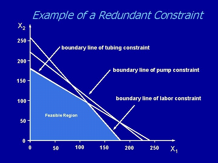
Example of a Redundant Constraint X 2 250 boundary line of tubing constraint 200 boundary line of pump constraint 150 boundary line of labor constraint 100 Feasible Region 50 0 0 50 100 150 200 250 X 1

Redundant Constraints (continued) As noted in the previous slide, the pump constraint is a redundant constraint and has no impact on the feasible region. In other words, we can usually eliminate the redundant constraint as it has no role in determining the feasible region.

Redundant Constraints (continued) Consider the following 2 constraints: X 1 >= 20 (1) X 1 >= 10 (2) Are these 2 constraints redundant? Yes, constraint (2) is redundant. It is identical to a scenario whereby I tell you must spend at least 20 dollars and add another statement you must spend at least 10 dollars. Which statement is binding? Clearly the first statement. Statement 2 is redundant.

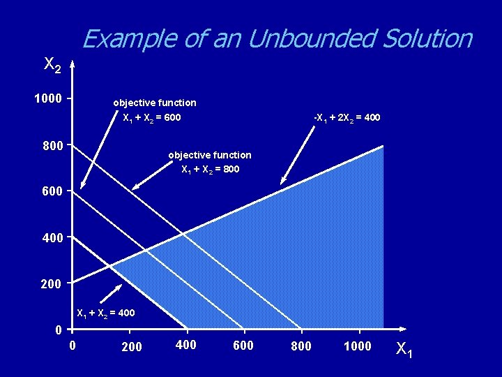
Example of an Unbounded Solution X 2 1000 objective function X 1 + X 2 = 600 800 -X 1 + 2 X 2 = 400 objective function X 1 + X 2 = 800 600 400 200 X 1 + X 2 = 400 0 0 200 400 600 800 1000 X 1

Unbounded Solution (continued) As the previous graph shows, we can technically make infinite profit as we can keep on pushing the level curve further and further. This situation came about due to the fact that the feasible solution has no boundary. Such problems should not arise in real life applications. If they do, this may signal an error in formulating the problem.

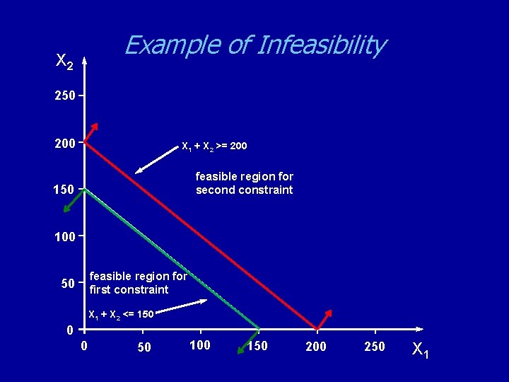
Example of Infeasibility X 2 250 200 X 1 + X 2 >= 200 feasible region for second constraint 150 100 feasible region for first constraint 50 X 1 + X 2 <= 150 0 0 50 100 150 200 250 X 1

Infeasibility (continued) As the previous graph shows, there is no way of being able to simultaneously satisfy both constraints. If that occurs in a real life application, this is a signal that the problem was formulated incorrectly.

Special Conditions in LP Problems Video Clip Now will be a good time to view the video clip titled “Special Conditions in LP Problems”.

Practice Problems § Under Week 1 Multimedia, there is a link under the heading Practice Problems that will provide you with further solutions to problems from your textbook using the graphical solution method.

End of Chapter 2