Linear Programming Review Characteristics of Linear Programming Models
- Slides: 15

Linear Programming (Review)

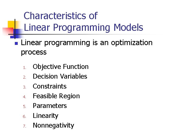
Characteristics of Linear Programming Models n Linear programming is an optimization process 1. 2. 3. 4. 5. 6. 7. Objective Function Decision Variables Constraints Feasible Region Parameters Linearity Nonnegativity

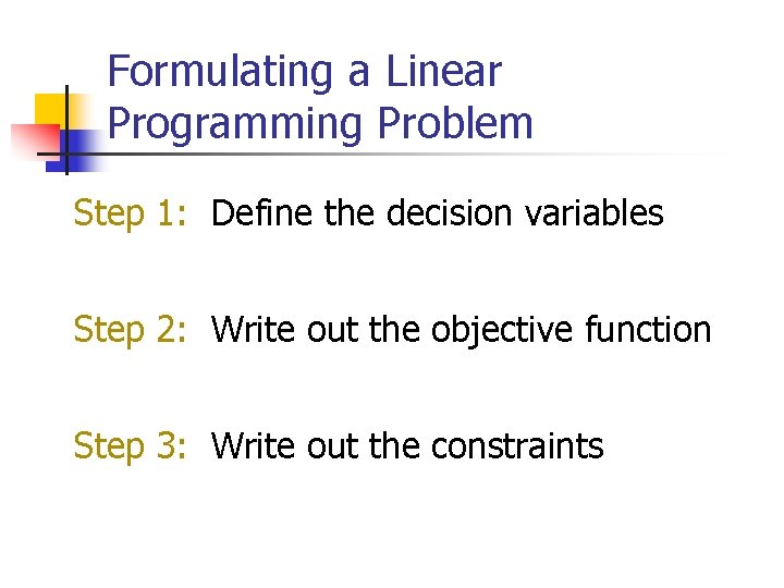
Formulating a Linear Programming Problem Step 1: Define the decision variables Step 2: Write out the objective function Step 3: Write out the constraints

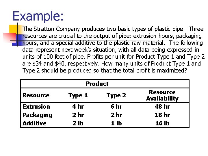
Example: The Stratton Company produces two basic types of plastic pipe. Three resources are crucial to the output of pipe: extrusion hours, packaging hours, and a special additive to the plastic raw material. The following data represent next week’s situation, with all data being expressed in units of 100 feet of pipe. Profits per unit for Product Type 1 and Type 2 are $34 and $40, respectively. How many units of Product Type 1 and Type 2 should be produced so that the total profit is maximized? Product Resource Type 1 Type 2 Extrusion Packaging Additive 4 hr 2 lb 6 hr 2 hr 1 lb Resource Availability 48 hr 16 lb

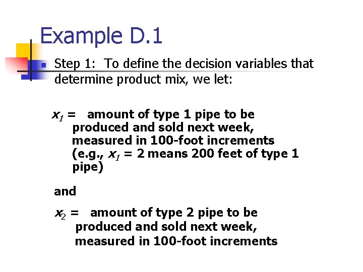
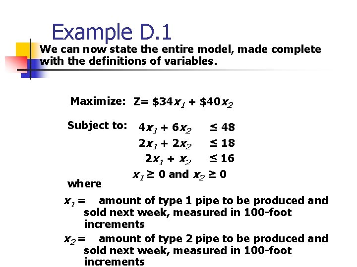
Example D. 1 n Step 1: To define the decision variables that determine product mix, we let: x 1 = amount of type 1 pipe to be produced and sold next week, measured in 100 -foot increments (e. g. , x 1 = 2 means 200 feet of type 1 pipe) and x 2 = amount of type 2 pipe to be produced and sold next week, measured in 100 -foot increments

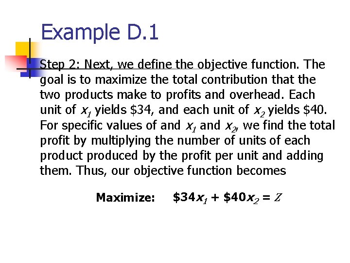
Example D. 1 n Step 2: Next, we define the objective function. The goal is to maximize the total contribution that the two products make to profits and overhead. Each unit of x 1 yields $34, and each unit of x 2 yields $40. For specific values of and x 1 and x 2, we find the total profit by multiplying the number of units of each product produced by the profit per unit and adding them. Thus, our objective function becomes Maximize: $34 x 1 + $40 x 2 = Z

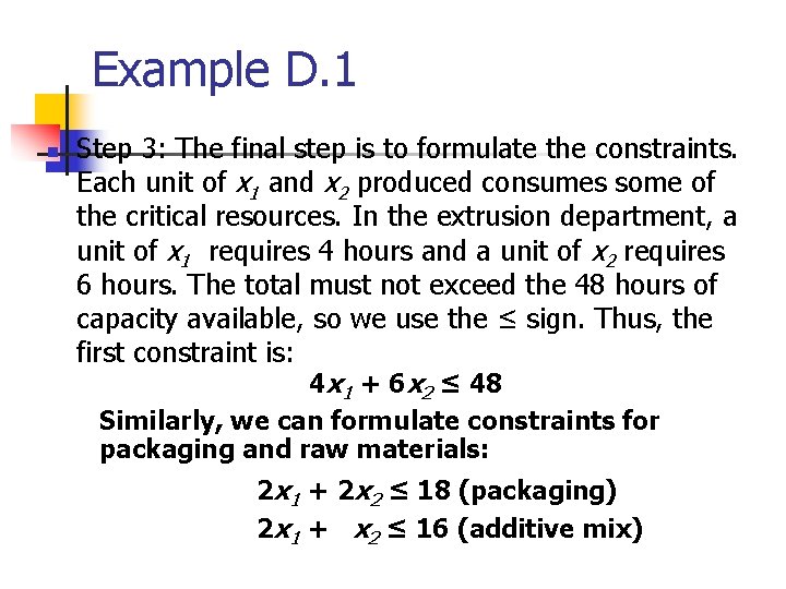
Example D. 1 n Step 3: The final step is to formulate the constraints. Each unit of x 1 and x 2 produced consumes some of the critical resources. In the extrusion department, a unit of x 1 requires 4 hours and a unit of x 2 requires 6 hours. The total must not exceed the 48 hours of capacity available, so we use the ≤ sign. Thus, the first constraint is: 4 x 1 + 6 x 2 ≤ 48 Similarly, we can formulate constraints for packaging and raw materials: 2 x 1 + 2 x 2 ≤ 18 (packaging) 2 x 1 + x 2 ≤ 16 (additive mix)

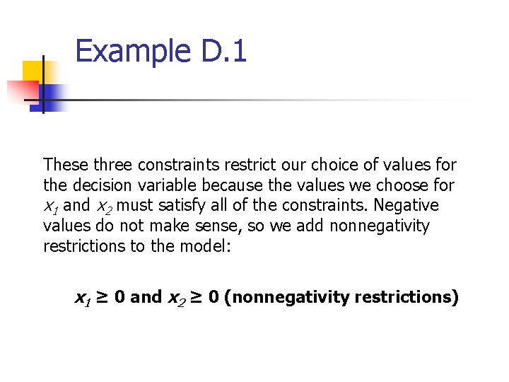
Example D. 1 These three constraints restrict our choice of values for the decision variable because the values we choose for x 1 and x 2 must satisfy all of the constraints. Negative values do not make sense, so we add nonnegativity restrictions to the model: x 1 ≥ 0 and x 2 ≥ 0 (nonnegativity restrictions)

Example D. 1 We can now state the entire model, made complete with the definitions of variables. Maximize: Z= $34 x 1 + $40 x 2 Subject to: where x 1 = 4 x 1 + 6 x 2 2 x 1 + 2 x 2 2 x 1 + x 2 x 1 ≥ 0 and x 2 ≤ 48 ≤ 16 ≥ 0 amount of type 1 pipe to be produced and sold next week, measured in 100 -foot increments x 2 = amount of type 2 pipe to be produced and sold next week, measured in 100 -foot increments

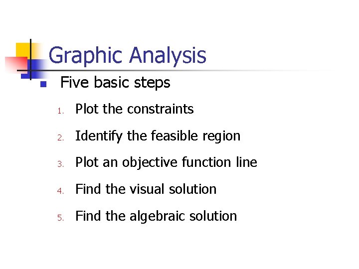
Graphic Analysis n Five basic steps 1. Plot the constraints 2. Identify the feasible region 3. Plot an objective function line 4. Find the visual solution 5. Find the algebraic solution

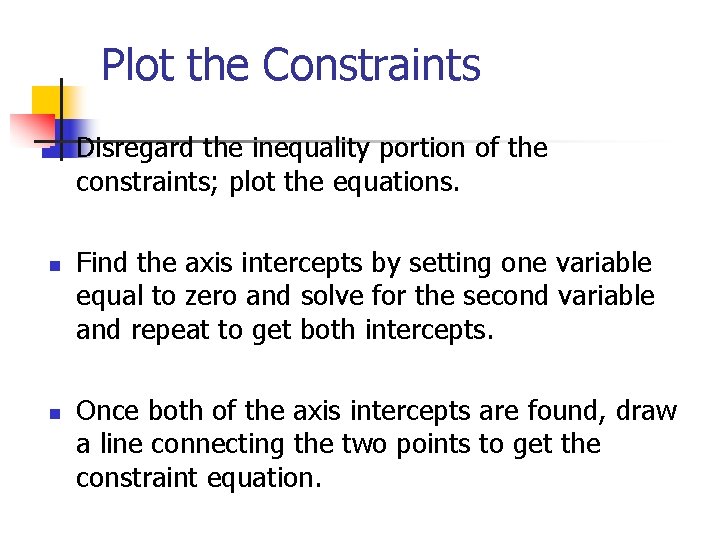
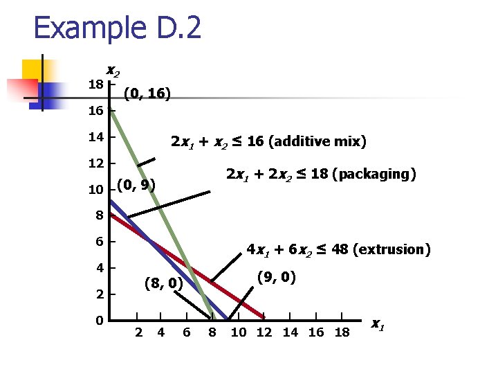
Plot the Constraints n n n Disregard the inequality portion of the constraints; plot the equations. Find the axis intercepts by setting one variable equal to zero and solve for the second variable and repeat to get both intercepts. Once both of the axis intercepts are found, draw a line connecting the two points to get the constraint equation.

Example D. 2 x 2 18 – (0, 16) 16 – 14 – 2 x 1 + x 2 ≤ 16 (additive mix) 12 – 2 x 1 + 2 x 2 ≤ 18 (packaging) 10 – (0, 9) 8– 6– 4 x 1 + 6 x 2 ≤ 48 (extrusion) 4– 2– 0– (9, 0) (8, 0) | | 2 4 6 8 | | | 10 12 14 16 18 x 1

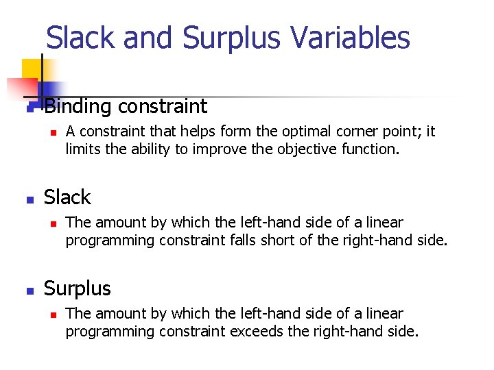
Slack and Surplus Variables n Binding constraint n n Slack n n A constraint that helps form the optimal corner point; it limits the ability to improve the objective function. The amount by which the left-hand side of a linear programming constraint falls short of the right-hand side. Surplus n The amount by which the left-hand side of a linear programming constraint exceeds the right-hand side.

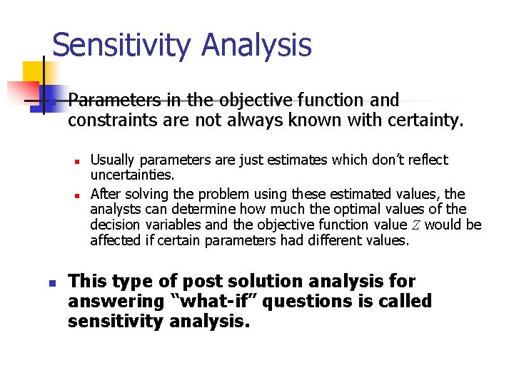
Sensitivity Analysis n Parameters in the objective function and constraints are not always known with certainty. n n n Usually parameters are just estimates which don’t reflect uncertainties. After solving the problem using these estimated values, the analysts can determine how much the optimal values of the decision variables and the objective function value Z would be affected if certain parameters had different values. This type of post solution analysis for answering “what-if” questions is called sensitivity analysis.

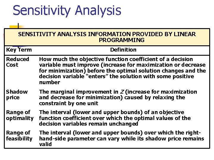
Sensitivity Analysis SENSITIVITY ANALYSIS INFORMATION PROVIDED BY LINEAR PROGRAMMING Key Term Definition Reduced Cost How much the objective function coefficient of a decision variable must improve (increase for maximization or decrease for minimization) before the optimal solution changes and the decision variable “enters” the solution with some positive number Shadow price The marginal improvement in Z (increase for maximization and decrease for minimization) caused by relaxing the constraint by one unit Range of optimality The interval (lower and upper bounds) of an objective function coefficient over which the optimal values of the decision variables remain unchanged Range of feasibility The interval (lower and upper bounds) over which the righthand-side parameter can vary while its shadow price remains valid